 Credit: John Bryant.  Flowers of the hazel tree. The large showy catkins are the male flowers. The female flowers are much smaller; one has opened beside the left-hand group of catkins. Credit: John Bryant. Flowers of the hazel tree. The large showy catkins are the male flowers. The female flowers are much smaller; one has opened beside the left-hand group of catkins. Credit: John Bryant. John writes … The heading of this blog post takes us back to the last words of my previous outing on these pages in which I wrote about the role of cold weather in regulating aspects of plant growth and development. Seeds of most plants growing in cool temperate regions are dormant – unable to germinate – when they are shed from the parent plant. In many species, dormancy is broken by an exposure to cold conditions, as I discussed in more detail in May. As also mentioned in that previous post, this is equally true of leaf and flower buds in biennial and perennial plants: in technical terms, the buds have to undergo a period of vernalisation (you will probably already know the word vernal which refers to things that happen in Spring such as the vernal equinox). Recent work by Prof Caroline Dean and Prof Martin Howard at the John Innes Centre in Norwich has started to unravel the mechanisms involved in vernalisation of flower buds. In autumn, the flower buds are dormant because the flowering process is held in check by the activity of a repressor gene. The activity of the repressor gene is sensitive to cold and so, during the winter, the gene is slowly switched off and eventually the genes that regulate flowering are able to work. OK then, plants have avoided leaf bud-burst or flowering at an inappropriate time but as Spring arrives, what is it that actually stimulates a tree to come into leaf or induces flowering in a biennial or perennial plant? Spring is characterised by several changes in a plant’s environment but the two most important are the increasing daytime temperature and the steady, day-by-day increase in daylength. In respect of temperature, it is clear that it is the major trigger for Spring-flowering plants. It is often said that Spring comes much earlier than it used to (even though, astronomically, the date of the equinox remains unchanged!). That observation was one of the catalysts for my writing these two blog posts and it has now been borne out by the data. In a recent research project carried out at Cambridge, on the effects of climate change, it was shown that in a range of 406 Spring-flowering trees, shrubs and non-woody plants, flowering now occurs a month earlier than it did in the mid-1980s (1). This ties in with my memories of Spring in Cambridge (I hope you’ll excuse a bit of reminiscing): when I was a student, the banks of the Cam were decorated with crocus flowers at the end of the Lent term, before we went home for Easter; when we came back for the summer term, it was daffodils that dominated the same banks. Now, the crocuses flower in the middle of the Lent term and the daffodils are in bloom at the end of that term.  The mathematical bridge at Queens’ College, Cambridge. This picture was taken in high summer but in spring, the displays of flowers (crocuses and daffodils) on the bank beyond the bridge have been good indicators of the earlier flowering dates referred to in the text. Credit: John Bryant. I will return to the induction of flowering later but now want to think about trees and shrubs coming into leaf. The situation is nicely illustrated by the old saying about oak (Quercus robur & Quercus petrea) and ash (Fraxinus excelsior): ‘Ash before Oak, we’re in for a soak; Oak before Ash, we’re in for a splash’. In colder, wetter Springs, oak budburst was delayed in comparison to ash and, in thinking about the weather, a cold wet Spring was believed to presage a wet summer (a ‘soak’). The folklore illustrates that budburst in oak is temperature-dependent. But what about ash? Its coming into leaf occurs at more or less the same time each year because the main trigger is increasing day-length. Thus, plants (or at least ash trees) have a light detection mechanism that can in some way measure the length of the light period. I need to add that because of climate change, these days, oak is nearly always before ash in respect of leaf production.
Going back to the nineteenth century, Darwin’s experiments on the effects of unilateral illumination clearly showed that plants bent towards the light because of differences in growth rate between the illuminated and non-illuminated side (2). This phenomenon is known as phototropism and shows that light can affect plant growth in a way not directly connected with photosynthesis. This added to previously established knowledge that plants grown in the dark or in very deep shade grew tall and spindly (‘etiolated’) and made little or no chlorophyll. Transfer of etiolated plants into the light slowed down the vertical growth rate and also led to the synthesis of chlorophyll, again showing that light can affect plant growth and development.  The main building at the Beltsville Agricultural Research Centre, Beltsville, Maryland, USA (I have visited the Centre and can reliably state that it, and the work done therein, are as impressive as it looks!). Credit: USDA/ARS.  Stick and ribbon representation of the structure of phytochrome. Credit: Yang, X., et al (2009) (3). Stick and ribbon representation of the structure of phytochrome. Credit: Yang, X., et al (2009) (3). These phenomena, and many others, lead us to think that plants must possess light receptors which are able to transduce the perception – and even quantification – of light into effects on growth. Further, these days we would say the effects on growth indicate effects on the expression of genes that control growth. The role of chlorophyll as a photo-reactive molecule, active in photosynthesis, was well known but the effects I am describing cannot be ascribed to chlorophyll since they can occur in its absence. The first of these non-chlorophyll photo-reactive molecules was discovered at the famous Beltsville Agricultural Research Centre in Beltsville, Maryland, USA where Sterling Hendricks and Harry Borthwick showed that red light was particularly effective in promoting several light-dependent developmental processes and that this promotion was reversed by far-red light. They proposed that plants contained a photo-reversible light-detecting molecule that was responsible for transduction of the perception of light into effects on growth and development. Cynics named this as yet unknown light receptor a ‘pigment of our imagination’ but Hendricks and Borthwick were proved right in 1959, when a pigment which had the predicted properties was identified by Warren Butler and Harold Siegelman. Butler called the pigment phytochrome which simply means plant colour or plant pigment. Over subsequent decades it has become clear that plants possess several subtly different variants of phytochrome, each with a specific role and there is no doubt that these are major regulators of the effects of light on plant growth and development. However, as research progressed, it became apparent that not all the effects of light could be attributed to photoreception in the red/far-red region of the spectrum. There must be others, particularly sensitive to light at the blue end of the spectrum (as Charles Darwin had suggested in the 1880s!). At the time of detailed analysis of the effects of blue light, the receptors were unknown – and hence given the name cryptochrome – hidden colour/pigment. Three cryptochrome proteins were eventually identified in the early 1980s. And there’s more! The overall situation is summarised in the diagram which is taken from a paper by Inyup Paik and Enamul Huq (4). It is clear that plants are able to respond to variations in light quality and intensity right across the spectrum. They cannot move away from their light environment but have evolved mechanisms with which to respond to it.  Light receptors in plants. That brings me back to flowering. While there is no doubt that many spring-flowering plants are responsive mainly to ambient temperature (as described earlier) and are thus neutral with regard to day-length, there are many plants which have specific day-length requirements. These are typified by summer-flowering plants such as sunflower (Helianthus annus) and snapdragon (Antirrhinum) which need n days in which daylight is longer than 12 hours (n differs between different species of long-day plants). Similarly, plants that flower in late summer or autumn, such as Chrysanthemum require n days in which there are fewer than x hours of daylight. Note that x may be above 12 hours but the key requirement is that days are shortening.  Flower of Sunflower (Helianthus annuus) accompanied by a White-tailed Bumblebee and a Red Admiral butterfly. Credit: John Bryant. So, the next time you are outside and thinking about your light environment (will it be sunny or cloudy?), just stop to ponder about the marvellous light response mechanisms that are happening in the plants all around you. John Bryant Topsham, Devon July 2024  PS: For those who want to read more about plant function and development, this book has been highly recommended! (1) Ulf Büntgen et al (2022), Plants in the UK flower a month earlier under recent warming
(2) As published in his 1880 book The Power of Movement in Plants. (3) Yang, X., et al (2009). (4) Inyup Paik and Enamul Huq (2019), Plant photoreceptors: Multi-functional sensory proteins and their signalling networks.
0 Comments
Graham writes ... Those of you who are regular visitors to this blog page may recall a post (1) in August 2023 when the so-called ‘Crisis in Cosmology’, or more formally what the cosmologists call ‘the Hubble tension’, was introduced and discussed. If you are not, then may I suggest that you have a read of the previous post to get a feel for the nature of the issue raised? Also please note that some sections of the previous post have been repeated here to make a coherent story. It concerns the value of an important parameter which describes the current rate of expansion of the Universe called Hubble’s constant, which is usually denoted by Ho (H subscript zero). This is named after Edwin Hubble, the astronomer who first experimentally confirmed that the Universe is expanding. The currently accepted value of H0 is approximately 70 km/sec per Megaparsec.  Edwin Hubble, and his famous pipe! Credit: Public Domain and Space Telescope Science Institute (STScI) (background image). As discussed in the book (2) (pp. 57-59), Hubble discovered that distant galaxies were all moving away from us, and the further away they were the faster they were receding. This is convincing evidence that the Universe is, as a whole, expanding (2) (Figure 3.4). The value of H0 above says that speed of recession of a distant galaxy increases by 70 km/sec for every Megaparsec it is distant. As explained in (1), a Megaparsec is roughly 3,260, 000 light years. Currently there are two ways to establish the value of Ho. The first of these, that is sometimes referred to as the ‘local distance ladder’ (LDL) method, is the most direct and obvious. This is essentially the process of measuring the distances and rates of recession of many galaxies, spread across a large range of distances, to produce a plot of points as shown below. The ‘slope of the plotted line’ gives the required value of Ho.  The slope of the best fit line gives the value of Hubble's constant. Credit: Rebecca Smethurst.  Max Planck. Credit: Public Domain Max Planck. Credit: Public Domain The second method employs a more indirect technique using the measurements of the cosmic microwave background (CMB). As discussed in the book (2) (pp. 60-62) and in the May 2023 blog post, the CMB is a source of radio noise spread uniformly across the sky that was discovered in the 1960s. At that time, it was soon realised that this was the ‘afterglow’ the Big Bang. Initially this was very high energy, short wavelength radiation in the intense heat of the early Universe, but with the subsequent cosmic expansion, its wavelength has been stretched so that it currently resides in the microwave (radio) part of the electromagnetic spectrum. The most accurate measurements we have of the CMB was acquired by the ESA Planck spacecraft , named in honour of the physicist Max Planck who was a pioneer in the development of quantum mechanics (as an aside, I couldn’t find a single portrait of Max smiling!). The ‘map’ of the radiation produced by the Planck spacecraft is partially shown below, projected onto a sphere representing the sky. The temperature of the radiation is now very low, about 2.7 K (3), and the variations shown are very small – at the millidegree level (4). The red areas are the slightly warmer, denser regions and the blue slightly cooler. This map is a most treasured collection of cosmological data, as it represents a detailed snap-shot of the state of the Universe approximately 380,000 years after the Big Bang, when the cosmos became transparent to the propagation of electromagnetic radiation.  The Planck spacecraft. Credit: ESA  Tiny temperature variations in the Cosmic Microwave Background captured by the ESA Planck spacecraft, projected onto a sphere representing the sky. Credit: ESA To estimate the value of H0 based on using the CMB data, cosmologists use what they refer to as the Λ-CDM (Lambda-CDM) model of the Universe (5) – this is what I have called ‘the standard model of cosmology’ in the book (2) (pp. 63 – 67, 71 – 76). The idea is that of using the CMB data as the initial conditions, noting that the ‘hot’ spots in the CMB data provide the seeds upon which future galaxies will form. The Λ-CDM model is evolved forward using computer simulation to the present epoch. This is done many times while varying various parameters, until the best fit to the Universe we observe today is achieved. This allows us to determine a ‘best fit value’ for H0 which is what we refer to as the CMB value. For those interested in the detail, please go to (1). The ‘crisis’ referred to above arose because the values of Ho, determined by each method, do not agree with each other, Ho = 73.o km/sec per Mpc (LDL), Ho = 67.5 km/sec per Mpc (CMB).  The 'evolution' of values of Ho since 2000. Credit: Jian-Ping Hu & Fa-Yin Wang, Hubble Tension: The evidence of new physics, 2023. Not only that, but the discrepancy is statically very significant, with no overlap of the estimated error bounds of the two estimates. So how can this mismatch between the two methodologies be resolved? It was soon realised that the implications of this disparity was either (a), the LDL method for estimating cosmic distances is flawed, or (b), our best model of the Universe (the Λ-CDM model) is wrong. Option (b) on the face of it sounds like a bit of a disaster, but since the birth of science centuries ago this has been the way that it makes progress. The performance of current theories is compared to what is going on in the real world, and if the theory is found wanting, it is overthrown and a new theory is developed. And in the process of course there is the opportunity, in this case, to learn new physics.  The James Webb Space Telescope (JWST). Credit: NASA, ESA, CSA Looking at the options, it would seem that the easier route is to check whether we are estimating cosmic distances accurately enough. Fortunately, we have a shiny new spacecraft available, that is, the James Webb Space Telescope (JWST), to help in the task. When I described the LDL method of estimating Ho above, it looks pretty straight forward, but it is not as easy as it sounds – measuring huge distances to remote objects in the Universe is problematic. The metaphor of a ladder is very apt as the method of determining cosmological distances involves a number of techniques or ‘rungs’. The lower rungs represent methods to determine distances to relatively close objects, and as you climb the ladder the methods are applicable to determining larger and larger distances. The accuracy of each rung is reliant upon the accuracy of the rungs below, so we have to be sure of the accuracy of each rung as we climb the ladder. For example, the first rung may be parallax (accurate out to distances of 100s of light years), the second rung may be using cepheid variable stars (2) (p. 58) (good for distances of 10s of millions of light years), and so on. Please see (1) for details. The majority of these techniques involve something called ‘standard candles’. These are astronomical bodies or events that have a known absolute brightness, such as cepheid variable stars, and Type Ia supernovae (the latter can be used out to distances of a billions of light years). The idea is that if you know their actual brightness, and you measure their apparent brightness as seen from Earth, you can estimate their distance. It is also interesting to note that a difference of 0.1 magnitude in the absolute magnitude of a ‘standard candle’, due to a discrepancy in estimating its distance, can lead to a 5% difference in the value of Ho. In other words, a value of Ho = 73 versus Ho = 69! It would seem the route of investigating the accuracy of estimating cosmic distances is fertile ground for a variety of reasons.  Wendy Freedman of the University of Chicago. Credit: Wendy Freedman and American Physical Society. Wendy Freedman of the University of Chicago. Credit: Wendy Freedman and American Physical Society. And this is exactly what Wendy Freedman, and her team of researchers, at the University of Chicago did. However, I should say that the results that now follow are not peer-reviewed, and therefore may change. The story henceforth is based on a 30-minute conference paper presentation at the American Physical Society meeting in April 2024. Interestingly, the title of her paper was “New JWST Results: is the current tension in Ho signalling new physics?”, which suggests that the original intention, at the time of the submission of the paper’s title and abstract, was to focus on objective (b) as mentioned above – in other words, looking at the implications of the standard model of the Universe being wrong. But in fact the focus is on (a) – an investigation of the accuracy of measuring distances. I can identify with this – when the conference deadline is so early that you’re not sure yet where your research is going! So, what did Freedman’s team do and achieve? They used two different ‘standard candles’ to recalibrate the distance ladder with encouraging results. The first of these are TRGB (Tip of the Red Giant Branch) stars. Without going into all the details, this technique assumes that the brightest red giant stars have the same luminosity and can therefore be used as a ‘standard candle’ to estimate galactic distances. The second class is referred to as JAGB (J-region Asymptotic Giant Branch) stars that are a class of carbon-rich stars that have near-constant luminosities in the near-infrared part of the electromagnetic spectrum. Clearly, these are useful as standard candles, and are also good targets for the JWST which is optimised to operate in the infrared. The team observed Cepheid variable, TRGB and JAGB stars in galaxies near enough for the JWST to be able to distinguish individual stars to determine the distances to these galaxies. Encouragingly, the results from each class of object gave consistent results for the test galaxies. Once a reliable distance to a particular galaxy was found, the team was able to recalibrate the supernova ‘standard candle’ data, which could then be used to re-determine the distances to very distant galaxies. After all that, they were able to recalculate the current expansion rate of the Universe as Ho = 69.1 ± 1.3 km/sec per Mpc The results of the study are encapsulated in the diagram below, which shows that the new result agrees with the CMB data calculation (labelled ‘best model of the Universe result’ in the diagram) within statistical bounds.  The value of Ho in units of km/sec per Mpc. Left is the existing CMB value, centre is the LDL value derived by the new (Freedman) study, and far right is the old LDL value based on Hubble space telescope data. Credit: Wendy Freedman and the American Physical Society. So, is that the end of the story? Well, as regards this study, it is yet to be peer-reviewed so things could change. Another aspect is that the apparent success here may encourage other groups to look back at their (predominately Hubble Telescope) data to recalibrate their previous estimates of galactic distances. So, I think this has a long way to run yet, but for now the Freedman Team should be congratulated in their efforts to ease the so-called ‘crisis in cosmology’!
Graham Swinerd Southampton, UK June 2024 (1) Blog post August 2023, www.bigbangtobiology.net. (2) Graham Swinerd & John Bryant, From the Big Bang to Biology: where is God?, Kindle Direct Publishing, November 2020. (3) The Kelvin temperature scale is identical to the Celsius scale but with zero Kelvin at absolute zero (-273 degrees Celsius). Hence, for example, water freezes at +273 K and boils at +373 K. (4) A millidegree is 1 thousandths of a degree. (5) Here CDM stands for cold dark matter, and the Greek upper-case Lamba (Λ) refers to Einstein’s cosmological constant, which governs the behaviour of dark energy.  Bluebells at Ripley, North Yorkshire. Credit: John Bryant. John writes … It’s all about the tilt. As we have mentioned before, Earth is a planet with ‘added interest’, namely the existence of different seasons, caused by the tilt in its axis (the 'obliquity of the ecliptic'), relative to the orbit plane, as shown in the picture below. As we move from the Equator towards the poles, the greater are the inter-seasonal differences in temperature and daylength. Indeed, at the poles, daylength varies from total darkness around the winter solstice to 24 hours of daylight around the summer solstice.  The Earth's rotational axis is not normal to the orbit plane, and it is this axial tilt that produces the seasonal variations. Credit: Source unknown. But we have a problem. In northern Europe, Spring is the most spectacular season, with the very obvious environmental change from the mainly brown hues of winter to the vibrant greens of new leaves and the range of glorious colours of myriad Spring-flowering plants. The soundscape becomes punctuated by birdsong and there is a general impression that the natural world is waking up. But this typifies the problem alluded to in the sub-heading. We think of natural selection as the selection of genetic variants that are best suited to their environment, leading to greater reproductive success. However, the environment is not constant but is subject to the seasonal variations that I have already alluded to, albeit that those variations are regular in the annual cycle. Thus, organisms living in, for example Finland, are subject to very different climatic pressures from those living in, for example, Kenya (I do not intend to discuss the changes in distribution and location of landmasses over geological time – this adds another, albeit very long-term perspective to the discussion). In this post and in my next contribution (probably in July), I want to discuss some of the features of various plants and animals that enable them to flourish in regions with significant seasonal variations.  Spring greens at Dove Cottage, Grasmere. Credit: John Bryant. Out in the cold. Moving quickly from Spring to Autumn, think of a tree, growing in northern Europe, that has produced seeds in September or October. The weather is still warm, warm enough to support seed germination and early seedling growth. However, the seeds do not germinate even when conditions seem ideal. We say that the seeds are dormant. Now let us move forward to the start of the new year. The weather is cold, the temperature may be below 0°C (depending on where you are) and indeed, there may be snow on the ground. These are not ideal conditions for young seedlings and thus it is a good thing that those seeds did not germinate.  Norway Maple tree. Credit: British Hardwood Tree Nursery. Allow me now to introduce the Norway Maple (Acer platanoides), a beautiful tree that has been planted in many parks in the UK. There is a particularly fine specimen in Ashton Park, Bristol. Earlier in my career, I and Dr Robert Slater studied the regulation of genes in relation to dormancy and germination in this species. It was already known that in order to break the dormancy, seeds needed to be kept moist for about 100 days at temperatures of 5°C or lower (a process known as stratification). Only then are the seeds able to respond when conditions such as soil temperature become favourable for germination. This means that in many parts of its range, established after the most recent glaciation, the seeds of Norway Maple rarely or never germinate and that includes specimens planted as ornamentals in parks in southern Britain. Further, this problem (for the tree) is exacerbated by climate change. 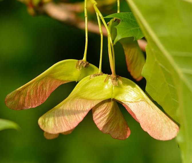 ‘Helicopter’ seeds of Norway Maple. Credit: Gardener’s Path (1). ‘Helicopter’ seeds of Norway Maple. Credit: Gardener’s Path (1). One of the things that happens during stratification is a change in the ratio of the concentrations of growth inhibitory hormones to concentrations of growth-promoting hormones. The changing ratio is in effect a measure of the length of the cold exposure. One of our key findings is that the genes associated with germination growth are not active until an appropriate ratio of growth regulators has been reached; thus we saw a flurry of gene activity at the end of the period of stratification. I need to say that Norway Maple seeds are not unique in requiring exposure to low temperatures before they can germinate. The seeds of many plant species native to north temperate regions, including the region’s tree species, exhibit the same trait, although few require a cold exposure as long as that required by the Norway Maple. Further, it is not only seeds that require a cold exposure before becoming active. Think now of biennial plants, plants that flower in the second of their two years of life. The buds which give rise to flowers in year-two will only do so after the plant has gone through a cold period; exposure to cold thus primes the floral buds to become active, a process which is known as vernalisation. Thus in my garden, the Purple Sprouting Broccoli plants that I am growing will not produce their purple sprouts (i.e., flowering shoots) until next Spring.
In summary, the seeds and plants that I have described cannot respond to the increasing ambient temperatures in Spring until they have experienced (and ‘measured’ that experience) the harsher conditions of the previous winter. Natural selection has thus led to the development of mechanisms that faciltate flourishing in areas with marked seasonal variation. ‘For everything, there is a season’ John Bryant Topsham, Devon May 2024 (1) https://gardenerspath.com/ Graham and John write ...  Welcome to the Lee Abbey Estate. Credit: Marion Swinerd. Welcome to the Lee Abbey Estate. Credit: Marion Swinerd. We co-hosted the 6th Lee Abbey conference in the ‘Big Bang to Biology’ series during the week of 18-22 March 2024. This week coincided with the Spring Equinox, heralding the beginning of Spring, presenting a wonderful opportunity to witness once again the renewal of the natural world. And what a great place to do it! Lee Abbey is a Christian retreat, conference and holiday centre situated on the North Devon coast near Lynton, which is run by an international community of predominantly young Christians. The main house nestles in a 280-acre (113 hectare) estate of beautiful farmland, woodland and coastal countryside, with its own beach at Lee Bay. The South West Coast Path passes through the estate and the Exmoor National Park is just a short drive away. The meeting took place before the Springtime clock change so that nightfall occurred at a reasonable time (not too late) in the evening. However, Graham’s one disappointment during the week was that cloud obscured the amazing night sky each evening! The site is on the edge of the Exmoor National Park Dark Sky Reserve.  Lee Abbey, with the dramatic coastal and rock scenery of the the Valley of Rocks beyond. Credit: Graham Swinerd.  The Conference venue, the main Lee Abbey House, on a cold, sunny March morning. Credit: Graham Swinerd.  We were pleased to welcome over 50 guests to the conference, who had booked in for a Science and Faith extravaganza. One of the joys of Lee Abbey is that speakers and delegates share the whole experience; meeting, eating and talking together for the whole week. This group of guests were a delight, which made the week a pleasure, coming as they did with an enthusiasm for the topic and a hunger to learn more and to share their own thoughts and experiences in discussion. It was also great to welcome Liz Cole back to the conference, with her new publication ‘God’s Cosmic Cookbook’ (1) – cosmology for kids!  The Lee Abbey Octagonal Lounge provided the perfect intimate meeting room for delegates and speakers. Credit: Jane Tompsett. The usual format for the conference is to have two one-hour sessions each morning. Graham kicked-off on Tuesday morning with sessions on the limitations of science (2) and the remarkable events of the early Universe (3), followed on Wednesday by a presentation on the fine-tuning and bio-friendliness of the laws that govern the Universe, combined with the story of his own journey of faith (4). During the second session, John followed on with a discussion of the equally remarkable events needed for the origin of life and for life’s flourishing on planet Earth (5). In the first session on Thursday morning, John posed a question – are we ‘more than our genes?’ involving a discussion of human evolution and what it means to be human (6). This was followed by an hour’s slot to give participants the opportunity to receive prayer ministry. The final event was an hour-long Q&A session in the late afternoon on Thursday. This was both a pleasure and a challenge for us speakers, with some piercing theological questions asked, as well as the scientific ones!  Castle Rock, Valley of Rocks. Credit: Graham Swinerd.  Valley of Rocks. Credit: Graham Swinerd. After the efforts of the mornings, delegates have free afternoons to enjoy the delights of the Lee Abbey Estate and the adjoining Valley of Rocks, followed by entertainment in the evening. Afternoon activities, such as local walks, are often arranged for guests by community. During the week additional events were also arranged. On Tuesday afternoon, guests were invited to visit the Lee Abbey farm by Estate Manager Simon Gibson to see the lambing and calving activities. Later that afternoon John offered an optional workshop on ‘Genes, Designer Babies and all that stuff’. Wednesday saw an entertaining presentation in the late afternoon by Dave Hopwood on Film and Faith, and on Thursday afternoon John led a guided walk to see the local flora, fauna and geology of the estate, Lee Bay and the Valley of Rocks.  Lambing season at Lee Abbey Farm. Credit: Marion Swinerd. Thank you to all who booked in and made the experience so worthwhile.
Graham Swinerd Southampton, UK John Bryant Topsham, Devon, UK 26 March 2024 (1) Elizabeth Cole, God’s Cosmic Cookbook: your complete guide to making a Universe, Hodder & Stoughton, 2023. (2) Graham Swinerd and John Bryant, From the Big Bang to Biology: where is God?, Kindle Direct Publishing, November 2020, Chapter 2. (3) Ibid., Chapter 3. (4) Ibid., Chapter 4. (5) Ibid., Chapter 5. (6) Ibid., Chapter 6. Graham writes ... 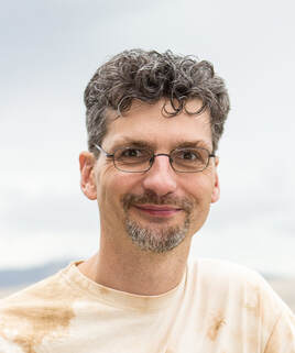 Christian Wolf. Credit: ANU. Christian Wolf. Credit: ANU. The real identity of what was thought to be a rather uninteresting nearby star was revealed in an article in Nature Astronomy on 19 February. The star, which is labelled J0529-4351, was first catalogued in a Southern Sky Survey dating back to 1980 (the rather uninteresting name is derived from the object’s celestial coordinates). Also, more recently, automated analysis by ESA’s Gaia spacecraft catalogued it as a star. The lead author of the article in Nature, Christian Wolf, is based at the Australian National University (ANU), and it was his team that first recognised the star’s true identity as a quasar last year, using the ANU’s 2.3 metre telescope at Siding Springs Observatory. As an aside, there is a relatively local link with this telescope, as it was once housed at Herstmonceux, Sussex as part of the Royal Greenwich Observatory. The true nature of the ‘star’ was further confirmed using the European Southern Observatory’s Very Large Telescope in Northern Chile. You can see the ANU’s press release here. 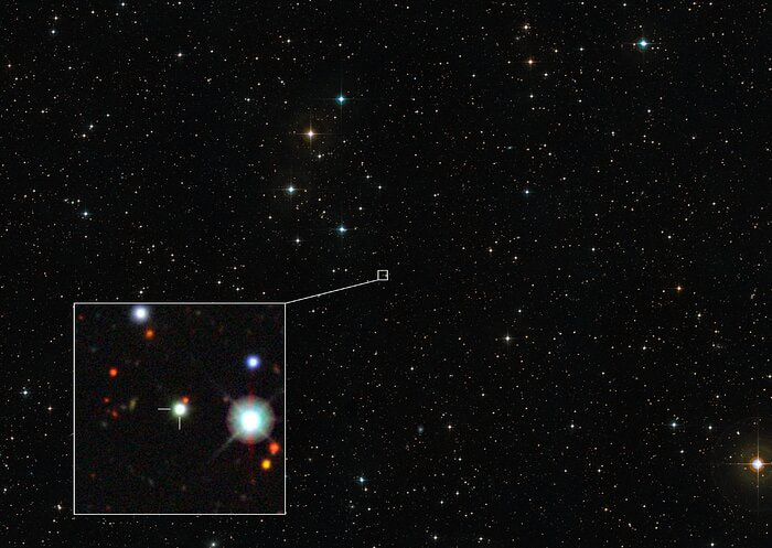 The quasi-stellar object J0529-4351 was first mis-identified at a uninteresting, relatively-nearby star. Credit: ESO. So, what’s a quasar you might ask? A quasar (standing for ‘quasi-stellar object’) is an extremely luminous active galactic nucleus. When first discovered in the 1960s, these star-like objects were known by their red-shift to be very distant from Earth, which meant that they were very energetic and extremely compact emitters of electromagnetic radiation. At that time, the nature of such an object with these characteristics was a subject for speculation. However, over time, we have discovered that super-massive black holes at the centre of galaxies are ubiquitous throughout the Universe. Indeed, we have one at the centre of our own Milky Way galaxy with a mass of 4 million Suns, just 27,000 light years away. So, when we observe a quasar, the light has taken billions of years to reach us, and we are seeing them as they were in the early Universe when galaxies were forming. In those early structures, ample gas and matter debris was available to feed the forming black holes, creating compact objects with a prodigious energy output. 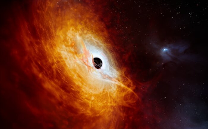 It's difficult to produce an artist's impression to do justice to the brightest object in the visible Universe! Credit: ESO. And this is what J0529-4351 turned out to be. This object’s distance was estimated to be 12 billion light years (a red-shift of z = 4), with a mass of approximately 17 billion Suns, hence dwarfing our Milky Way black hole. As black holes feed on the surrounding available material (gas, dust, stars, etc.) they form an encircling accretion disk, in which the debris whirlpools into the centre. Velocities of material objects in this disk approach that of light speed, and the emission from the quasar radiates principally from this spiralling disk. The accretion disk of J0529-4351 is roughly 7 light years in diameter, with the central blackhole consuming just over one solar mass per day. This gives the object an intrinsic brightness of around 500 trillion Suns, making it the brightest known object in the Universe. Hopefully, like me, you are awed at the characteristics of this monstrous black hole that provided this amazing light show 12 billion years ago! Apologies that this month’s blog is shorter than usual, mainly because of preparation work required for next month’s conference at Lee Abbey, Devon, UK (see information on the home page). For those booked in, we are really looking forward to meeting you all next month!
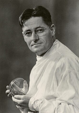
John has also been busy posting other item(s) of interest on our ‘Big Bang to Biology’ Facebook page. Graham Swinerd Southampton, UK February 2024  Picture credit: www.gblpharma.com John writes … A century (nearly) of antibiotics It is one of those things that ‘every school pupil knows’: Alexander Fleming discovered penicillin in 1928. At the time, he thought that his discovery had no practical application. However, in 1939, a team at Oxford, led by Howard Florey, started to work on purification and storage of penicillin and having done that, conducted trials on animals followed by clinical trials with human patients. The work led to its use amongst Allied troops in the World War II and, after the war, in more general medical practice. Its detailed structure was worked out by Dorothy Hodgkin, also at Oxford, in 1945 and that led to the development of a range of synthetic modified penicillins which are more effective than the natural molecule.
This leads us to think about penicillin’s mode of action: it works mainly by disrupting the synthesis of the bacterial cell wall which may in turn lead to the autolysis (self-destruction) of the cell. Other antibiotics have since been developed which target other aspects of bacterial metabolism. In my own research on genes, I have used rifampicin which inhibits the transcription (copying) of genes into messenger RNA (the working copy of a gene) and chloramphenicol which prevents the use of messenger RNA in the synthesis of proteins (1). However, antibiotics in the penicillin family are by far the most widely used (but see next section). 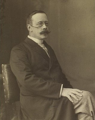 Hans Christian Gram (1853 -1938) Photograph by Niels Christian Hansen and Frantz Clemens Stephan Weller via Wikimedia Commons. Hans Christian Gram (1853 -1938) Photograph by Niels Christian Hansen and Frantz Clemens Stephan Weller via Wikimedia Commons. But there’s a problem Bacteria can be grouped according to whether they are ‘Gram-positive’ or ‘Gram-negative’. Hans Christian Gram was a Danish bacteriologist who developed a technique for staining bacterial cells – the Gram stain. Species which retain the stain, giving them a purple colour, are Gram-positive; species which do not retain the stain are Gram-negative. We now know that this difference is caused by differences in the cell’s outer layers. Gram-positive bacteria have a double-layered cell membrane (the plasma-membrane), surrounded by a thick cell wall; Gram-negative bacteria also have a double-layered plasma-membrane which is surrounded by a thinner cell wall and then another double-layered membrane. It is this structure that prevents the stain from entering the cells and which also leads to antibiotics in the penicillin family being totally or partially ineffective. Like many molecular biologists, I have used non-pathogenic strains of a Gram-negative bacterium, Escherichia coli (E .coli). It is the bacterial model used in research and has also been used to ‘look after’ genes which were destined for use in genetic modification. By contrast, pathogenic strains of this species can cause diarrhoea (‘coli’ indicates one of its habitats – the colon) while more seriously, some Gram-negative bacteria may cause pneumonia and sepsis. As already indicated, penicillin derivatives are mostly ineffective against Gram-negative bacteria and some of the effective antibiotics which have been developed have quite serious side effects. 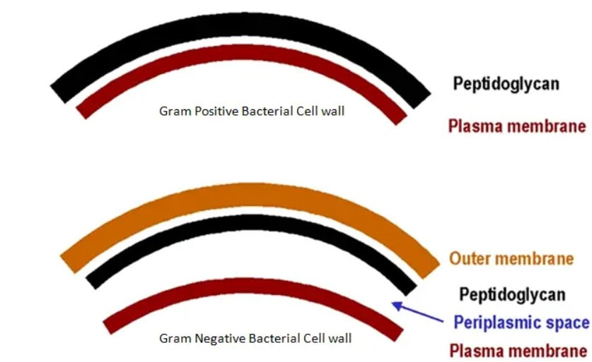 Simplified diagram showing the differences between the membranes and cell walls of Gram-positive and Gram-negative bacteria. The term ‘peptidoglycan’ refers to the cell wall (complex molecules called peptidoglycans make up the bulk of the wall). Picture from www.microbeonline.com. And an even bigger problem It is a truth universally acknowledged that an organism better adapted to an environment will be more successful than one that is less well adapted. This is of course a slightly ‘Austenesque’ way of talking about natural selection. Suppose then, that antibiotics are so widely used in medical, veterinary, or agricultural settings that they effectively become part of the environment in which bacteria live. Initially there will be a small number of bacteria that, for a number of reasons, are resistant to antibiotics. For example, some are able to de-activate a particular antibiotic and some can block the uptake of an antibiotic. Whatever the reason for the resistance, these resistant bacteria will clearly do better than the non-resistant members of the same species. The resistance genes will be passed on in cell division and the resistant forms will come to dominate the population, especially in locations and setting where antibiotics are widely used. And that, dear reader, is exactly what has happened. Antibiotic resistance is now widespread especially in Gram-negative, disease-causing bacteria, as is seen in the WHO priority list of 12 bacterial species/groups about which there is concern: nine of these are Gram-negative. The situation, already an emergency, is now regarded as critical in respect of three Gram-negative bacteria. Thinking about this from a Christian perspective, we might say that antibiotics are gifts available from God’s creation but humankind has not used those gifts wisely.  The WHO chart of the ‘dirty dozen’ – the most serious of the antibiotic resistant bacteria. But there is hope The growing awareness of resistance has catalysed a greatly increased effort in searching for new antibiotics. There are many thousands of organisms ‘out there’ remaining to be discovered, as is evident from a recent announcement from Kew about newly described plant and fungal species. It is equally likely that there is naturally occurring therapeutic chemicals, including antibiotics, also remaining to be discovered, perhaps even in recently described species (remembering that penicillin is synthesised by a fungus). There are also thousands of candidate-compounds that can be made in the lab. Concerted, systematic, computer-aided high throughput searches are beginning to yield results and several promising compounds have been found (2). Nevertheless, no new antibiotics that are effective against Gram-negative bacteria have been brought into medical or veterinary practice for over 50 years. However, things may be about to change. On January 4th, a headline on the BBC website stated ‘New antibiotic compound very exciting, expert says’ (3). The Guardian newspaper followed this with ‘Scientists hail new antibiotic that can kill drug-resistant bacteria.’ (4) The antibiotic is called Zosurabalpin and it was discovered in a high throughput screening programme (as mentioned earlier) that evaluated the potential of a large number of synthetic (lab-manufactured) candidate-compounds. In chemical terminology Zosurabalpin is a tethered macrocyclic peptide, an interesting and quite complex molecule. However, its most exciting features are firstly its target organisms and secondly its mode of action. Both of these are mentioned in the news articles that I have referred to and there is a much fuller account in the original research paper in Nature (5). 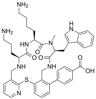 Structure of Zosurabalpin. Public domain. Referring back to the WHO chart, we can see that one of the ‘critical’ antibiotic-resistant bacteria is Carbapenem-resistant Acinetobacter baumannii (known colloquially as Crab). Carbapenem is one of the few antibiotics available for treating infections of Gram-negative bacteria but this bacterial species has evolved resistance against it (as described above). This means that it is very difficult to treat pneumonia or sepsis caused by Crab. The effectiveness of Zosurabalpin against this organism is indeed very exciting. Further, I find real beauty in its mode of action in that it targets a feature that makes a Gram-negative bacterium what it is. One of the key components of the outer membrane is a complex molecule called a lipopolysaccharide, built of sugars and fats. The antibiotic disrupts the transport of the lipopolysaccharide from the cell to the outer membrane which in turn leads to the death of the cell. 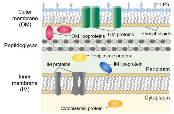 The outer layers of a Gram-negative bacterial cell in more detail, showing the inner membrane, the peptidoglycan cell wall and the outer membrane. The essential lipopolysaccharides mentioned in the text are labelled LPS. The new antibiotic targets the proteins that carry the LPS to their correct position. Diagram modified from original by European Molecular Biology Lab, Heidelberg. Zosurabalpin has been used, with a high level of success, to treat pneumonia and sepsis caused by A. baumannii in mice. Further, trials with healthy human subjects did not reveal any problematic side-effects. The next phase of evaluation will be Phase 1 clinical trials, the start of a long process before the new antibiotic can be brought into clinical practice. John Bryant Topsham, Devon January 2024 (1) For anyone interested in knowing more about how antibiotics work, there is a good description here: Action and resistance mechanisms of antibiotics: A Guide for Clinicians – PMC (nih.gov).
(2) As discussed here: Antibiotics in the clinical pipeline as of December 2022 | The Journal of Antibiotics (nature.com). (3) New antibiotic compound very exciting, expert says – BBC News. (4) Scientists hail new antibiotic that can kill drug-resistant bacteria | Infectious diseases | The Guardian. (5) A novel antibiotic class targeting the lipopolysaccharide transporter | Nature. Graham writes …  Credit: News18. The Nobel Prize in Physics 2023 has been awarded jointly to Anne L’Huillier of Lund University in Sweden, Pierre Agostini of Ohio State University in the USA and Ferenc Krausz of the Ludwig Maximilian University in Munich, Germany, for their experimental work in generating attosecond pulses of light for the study, principally, of the dynamics of electrons in matter. 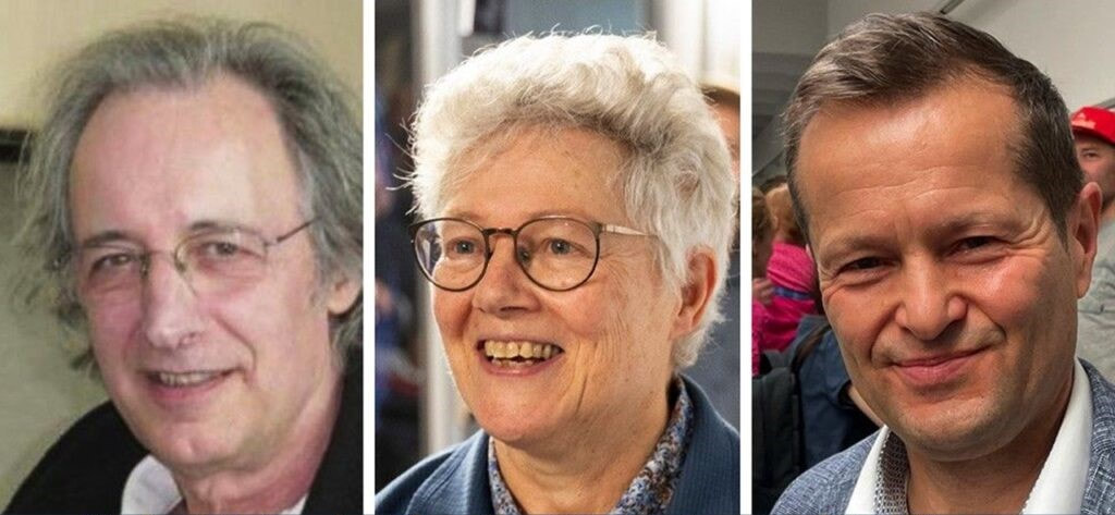 Nobel Laureates (L to R) Pierre Agostini, Anne L'Huillier and Ferenc Krausz. Credit: NEWS-DO. Effectively, the three university researchers have opened a new window on the Universe, and this will inevitably lead to new discoveries. Before we think about the applications of this newly-acquired technique, we need to explore the Nobel Laureates’ achievements in general terms. Firstly it would be good to know, what is an attosecond (as)? It is a very short period of time, which can be expressed in variety of ways, 1 as = a billion, billionths of a second, = 0.000 000 000 000 000 001 sec, or in ‘science-speak’, = 10^-18 sec. Whichever way you think of it, it is an unimaginably short period of time. Other observers reporting on this have pointed out that there are more attoseconds in one second than there are seconds of time since the Big Bang! I don’t know if that helps? In general terms, what the research has led to is the development of a ‘movie camera’ with a frame rate of the order of 10 million billion frames per second. Effectively this allows the capture of ‘slow-motion imagery’ of some of the fastest known physical phenomena, such as the movement of electrons within atoms. If we think about objects in the macroscopic world, generally things happen on timescales related to size. For example, the orbits of planets around the Sun take years, and the time it takes for a human being to run a mile is measured in minutes and seconds. Another macroscopic object that moves very rapidly is a humming bird. Or rather, while it hovers statically to consume plant nectar its wings need to flap around 70 times per second, which is once every 0.014 sec. Clearly if we had a movie camera with a frame rate of, say 25 per second then the bird’s wings would simply be a blur. To examine each wing beat in detail, to study how the bird achieves its steady hover, then a minimum of maybe 10 frames per flap would be required. So, something like, at least, 1,000 frames per second would be advised to allow an informative slow-motion movie of the bird’s physical movements. If we now consider the quantum world of particles and atoms, movements such as the dance of electrons in atoms are near-instantaneous. In 1925, Werner Heisenberg (one of the pioneers of quantum mechanics, and the discoverer of the now famous uncertainty principle) was of a view that the orbital motion of an electron is unobservable. In one sense he was correct. As a wave-particle, an electron does not orbit the atom in the same way as planets orbit the Sun. Rather physicists understand them as electron clouds, or probability waves, which quantify the probability of an electron being observed at a particular place and time. However, the odds of an electron being here or there change at the attosecond timescale, so in principle our attosecond ‘movie camera’ can directly probe electron behaviour. I’m sure that Heisenberg would have been delighted to learn that he had underestimated the ingenuity of 21st Century physicists. 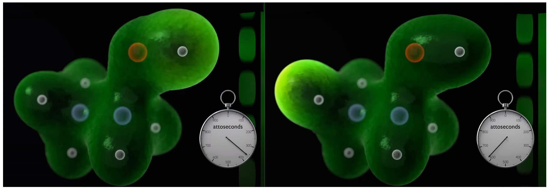 Electrons, or rather electron clouds, move around atoms and molecules with an attosecond timescale. Credit: PBS Space Time. However, the ‘movie camera’ we have been discussing, is not a camera in the conventional sense. Instead a laser beam with attosecond period pulses is brought to bear on objects of interest (such as atoms within molecules, or electrons within atoms) to illuminate their frenzied movements. But how is this achieved? L’Huillier team’s early work prepared the scene for attosecond physics. They discovered that a low frequency infra-red (heat radiation) laser beam passing through argon gas generated a set of additional high-energy “harmonics” – light waves whose frequencies are multiples of the input laser frequency. The idea of harmonics is a very familiar one in acoustics, and in particular those generated by musical instruments. The quality of sound that defines a particular instrument (its ‘timbre’) is determined by the combination of its fundamental frequency combined with its main harmonic frequencies. In music, the amplitude (or loudness) of the higher harmonics tends to decrease as the frequency increases, but one striking characteristic that L’Huillier found was that the amplitude of the higher harmonics in the laser light did not die down with rising frequency. The next step was to try to understand this observed behaviour. L’Huillier’s team set about constructing a theoretical model of the process, which was published in 1994 (1). The basic idea is that the laser distorts the electric-field structure within the argon atom, which allows an electron to escape. This liberated electron then acquires energy in the laser field and when the electron is finally recaptured by the atom it gives away the acquired energy in the form of an emitted photon (particle of light). This released energy generates the higher frequency harmonic waveforms. The next question was whether the light corresponding to the higher harmonic modes would interfere with each other to generate attosecond pulses? Interference is a commonly observed phenomenon, when two or more electromagnetic (or acoustic) wave forms are combined to generate a resultant wave in which the displacement is either reinforced or cancelled. This is illustrated in the diagram below. In this example, two wave trains with slightly differing frequencies are combined to produce the resultant waveform (this occurrence is called ‘beats’ in acoustics). Notice that the maximum outputs in the lower, combined wave train occur when the peaks in the original waves coincide, and similarly a minimum occurs when the peaks and troughs coincide to cancel each other out.  A simple example of interference between two wave trains. The waves combine to either increase or cancel the wave amplitude to produce the lower wave form. In the case of L’Huillier’s experiments, for interference to occur a kind of synchronisation between the emission of different atoms is required. If the atoms do not ‘collaborate’ with each other, then the output will be chaotic. In 1996 the team demonstrated theoretically that the atoms (remarkably) do indeed emit phased-matched light, allowing interference between the higher harmonics to occur, so opening the door to the prospect of attosecond physics. The image below illustrates the generation of attosecond pulses as a consequence of the interference between the various higher harmonic wave train outputs. 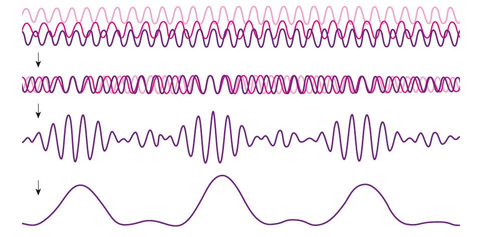 Top level shows a variety of higher harmonic waves, which are combined in the second level to give the resultant wave in level 3. This finally gives the sequence of pulses shown at the bottom of the figure. Over the subsequent years, physicists have exploited these detailed insights to generate attosecond pulses in the laboratory. In 2001, Agostini’s team produced a train of laser pulses, each around 250 as duration. In the same year, Krausz’s group used a different technique to generate single pulses, each of 650 as duration. Two years later, L’Huillier’s team pushed the envelope a little further to produce 170 as laser pulses. So, the question arises, what can be done with this newly acquired ‘super-power’? Well in general it will allow physicists to study anything that changes over a period of 10s to 100s of attoseconds. As discussed above, the first application was to try something that the physics community had long considered impossible – to see precisely what electrons are up to. In 1905 Albert Einstein was instrumental in spurring the early development of quantum mechanics with his explanation of the photoelectric effect. The photoelectric effect is essentially the emission of electrons from a material surface, as a result of shining a light on it. He later won the 1921 Nobel Prize in Physics for this, and it is remarkable that he did not receive this accolade for the development of the theory of general relativity, which could be considered to be his crowning achievement. Einstein’s explanation showed that light behaved, not only as a wave, by also as a particle (the photon). The key to understanding was that the numbers of photo electrons that were emitted from the surface was independent of the intensity of the light and but rather depended upon its frequency. This emission was considered to take place instantaneously, but Krausz’s team examined the process using attosecond pulses and could accurately time how long it took to liberate a photoelectron.  Agostini's experimental set up. Credit: PBS Space Time. The developments I have described briefly in this post suggest a whole new array of potential applications, from the determination of the molecular composition of a sample for the purposes of medical diagnosis, to the development of super-fast switching devices that could speed up computer operation by orders of magnitude – thanks to three physicists and their collaborators who explored tiny glimpses of time.
Graham Swinerd Southampton, UK December 2023 (1) Theory of high-harmonic generation by low-frequency laser fields, M. Lewenstein, Ph. Balcou, M. Yu. Ivanov, Anne L’Huillier, and P. B. Corkum, Phys. Rev. Vol. A 49, p. 2117, 1994.  Greetings and blessings of the season to you all from John and Graham. Please click on the picture. (Graham's choir is singing this blessing from the pen of Philip Stopford this Christmas season). Graham's December blog post on the 2023 Nobel Prize in Physics will be arriving soon ...
John writes ...  20-week foetus. Credit: Steve Allen Photography via Alamy. Introduction. Sickle-cell anaemia is a condition that occurs predominantly amongst people of Afro-Caribbean and Indian heritages. Eighty percent of cases occur in sub-Saharan Africa (see map) but we also note that, on a per capita basis, the Caribbean region has the second highest rate of occurrence (1). The name of the disease comes from the shape of the red blood cells which, instead of being round and squishy, are sickle-shaped and rather stiff. This means that they don’t travel so well through the smaller blood vessels which are thus prone to blockage, leading to a range of symptoms, including severe pain, as described in the NHS information page (2). Further, these aberrant red blood cells have a much shorter life in the body than normal red cells. This means that rates of cell production in the bone marrow may not keep up with the body’s needs, leading to anaemia. 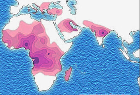 Distribution of sickle-cell disease in Africa and Eurasia. Credit: Muntuwandi at English Wikipedia, via GNU Free Documentation Licence. 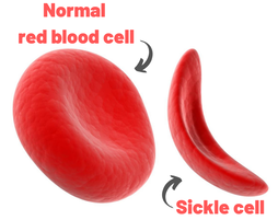 Normal and sickle-shaped red blood cells. Credit: public domain. Normal and sickle-shaped red blood cells. Credit: public domain. The sickle-shape of the red blood cells is caused by change in the structure of the oxygen-carrying protein, haemoglobin. Intriguingly, at normal oxygen concentrations, the oxygen-carrying capacity of the mutant haemoglobin is only slightly affected. However, it is when the protein ‘discharges’ its cargo of oxygen in the tissues where it is needed, that the change in its structure has its effect. The globin molecules stick together leading to the changes in the red cells that I mentioned earlier. 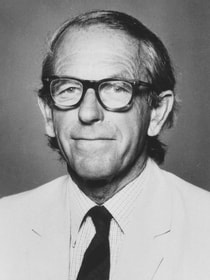 Fred Sanger. Credit: Public Domain Fred Sanger. Credit: Public Domain Some history. At this point we need to remind ourselves firstly that the building blocks of protein are called amino acids and secondly that the order of the building blocks (‘bases’) in DNA ‘tells’ the cell which amino acids to insert into a growing protein (Chapter 5 in the book). The order of bases in the DNA is thus the genetic code in which a group of three bases (a codon) corresponds to a particular amino acid and it is interesting that the biochemistry of haemoglobin has a significant role in our knowledge of this. Firstly, thanks mainly to the work of Fred Sanger in Cambridge, it was already possible in the late 1950s to work out the order of amino acids in protein. Sanger was awarded the 1958 Nobel Prize for Chemistry in recognition this work. Thus, the amino sequences of normal and sickle-cell haemoglobin could be compared and by 1959, Vernon Ingram, an American scientist working in Cambridge, had shown that the two differed by just one amino acid. In sickle-cell haemoglobin, a molecule of glutamic acid is replaced by a molecule of valine (3). Secondly, it was not long after, in 1961, that scientists started to crack the genetic code, a task that was completed by 1966. Marshall Nirenberg and Gobind Khorana were awarded the 1968 Nobel Prize for their major roles in this achievement. This meant that the presence of valine instead of glutamic acid in sickle-cell haemoglobin could be ascribed to a mutation in DNA in which the codon GAG is replaced the codon GTG (we recall that we often refer to the bases in DNA just by their initials, A, C, G, T). In other words, a mutation which involved the change of just one base was responsible for the aberrant behaviour of the mutant haemoglobin. GAG in DNA → Glutamic acid in protein GTG in DNA → Valine in protein This was the very first elucidation of a point mutation involving just one base which leads to the synthesis of a malfunctioning protein. It is worth reminding ourselves that this was achieved over a decade before Sanger (again!) published a method for sequencing DNA, a milestone which led to his receiving, in 1980, another Nobel Prize for Chemistry. Although other methods were developed at around the same time, the Sanger method was the first choice of most researchers, including me, from its arrival on the scene in 1977 until around 2010, when two much faster methods became widely adopted. In relation to sickle-cell disease, Sanger’s method was immediately used to sequence the normal and mutant globin genes, directly demonstrating the GAG to GTG change that had been deduced in previous research (as described above). Back to the womb. In the Bible, Nicodemus asked incredulously whether it was possible to return to his mother’s womb, with the strong implication that it was not (4). Of course, he was right. Here our figurative return to the womb involves looking at the haemoglobin circulating in the foetal blood stream. As in post-natal life, the haemoglobin has to pick up oxygen and deliver it round the body but from where does it get the oxygen? The only source available is the mother’s blood stream circulating through the placenta. The maternal and the foetal bloodstreams do not mix and so this oxygen capture occurs across cellular membranes. The transfer from the maternal to the foetal bloodstreams happens because foetal haemoglobin has a higher affinity (‘grabbing power’) for oxygen than maternal haemoglobin. It can therefore pull the oxygen from the mother’s bloodstream to the foetus’s bloodstream. If you find that hard to imagine, think of a magnet that has picked up some paper clips; if a stronger magnet is brought into the vicinity, it will ‘capture’ the paper clips from the weaker magnet (5). At birth, a remarkable genetic event starts to occur: the gene encoding foetal haemoglobin is down-regulated by the activity of a repressor gene (known as BCL11A) and the gene encoding adult haemoglobin is switched on. By the time an infant is about six months old, the red cells contain, almost exclusively, adult haemoglobin although most of us continue to make a tiny amount of foetal haemoglobin (about 1% of the total) throughout life. Furthermore, when we look at that small amount of persistent foetal haemoglobin it is clear that it does not carry the sickle-cell mutation, even in people with sickle-cell disease. Genome editing can cure sickle-cell disease. The gene-switching phenomenon that I describe above immediately raises the possibility of reversing the switch as a route to curing sickle-cell disease. Indeed, over the past two to three years there have been reports of the success of trials using exactly this approach. The story of one patient, Jimi Olaghere, is told in this BBC article: Sickle cell: ‘The revolutionary gene-editing treatment that gave me new life’ – BBC News.  Jimi Olaghere, cured of sickle-cell disease by the gene-editing procedure. Credit: Jimi Olaghere. In practice, the procedure is quite complex but the principle is clear. A patient’s bone marrow stem cells (from which blood cells are produced) are removed. Genome editing is used to inactivate both the mutant adult haemoglobin gene and the repressor that normally switches off the foetal haemoglobin gene. The bone marrow stem cells are put back in the patient who then starts producing foetal haemoglobin. We need to say at this point that because foetal haemoglobin is better at grabbing oxygen than adult haemoglobin it is also less good at releasing it out in the body’s tissues. This is not a problem for a foetus whose oxygen demands are not great but for a child or adult, this probably means that activities with high oxygen demand, including many sports, may be difficult (although golf is clearly possible). Nevertheless, it is obvious from the testimonies of patients like Jimi Olaghere that their lives are so much better after the treatment than before, including being able to play golf without the sickle-cell-associated pain. I started to compose this blog post on November 13th because I knew of the successful trials and I also learned that regulatory authorities in the USA, the EU and the UK were looking at the trials with a view to authorising the use of this gene-editing procedure in clinical practice. It was therefore very gratifying to turn on the BBC News on November 16th to hear that the UK’s Medicines and Healthcare Products Regulatory Agency (MHRA) had approved the procedure for treating both sickle-cell disease and thalassaemia (see below). This was also reported by several daily newspapers (6) and by New Scientist in its daily news (7). Thalassaemia. As mentioned above, the MHRA has also authorised the gene-editing procedure for use in treating another inherited haemoglobin disorder, thalassaemia, a move that was warmly welcomed by the Cyprus-based Thalassaemia International Federation (8). The name of the disease comes from the Greek word for sea and the name of the sea goddess, Thalassa (Θάλασσα) in Greek mythology. This is because people living around the eastern Mediterranean exhibit some of the highest incidences of thalassaemia; in an earlier publication (9) I describe programmes in Cyprus aimed at reducing the incidence of the disease. The seriousness of thalassaemia depends on which mutation or mutations a person has but for people with the most serious versions, life can be very difficult. I do not have the space here to describe the genetics or the symptoms in any more detail (see references for further information). However, I do want to emphasise that the trials of the gene-editing procedure described above also involved thalassaemia patients and were equally successful. A pause for thought. Overall response to this development has been very positive and rightly so: it is a brilliant use of excellent science. However, I want to pause for a moment to refer back to the opening paragraph. Eighty percent of cases of sickle-cell disease occur in sub-Saharan Africa with high incidences also seen in India and in the Caribbean region. The gene-editing-based treatment is very expensive, although in the UK, the USA and western Europe it is considered that, in cold accounting terms, the cost of this treatment is less than the lifetime costs of dealing with the medical needs of someone with sickle-cell disease or thalassaemia. That may be so but we still need to ask whether the treatment can be made available to the low and middle-income countries where the need is greatest.  David Liu. He and his research team at Harvard University were pioneers of DNA base-editing. Credit: Casey Atkins Photography, courtesy of the Broad Institute A look to the future. In my blog post for December 2022, I mentioned that a very accurate form of genome editing called DNA base-editing had been used to treat a teenage girl who had T-cell acute lymphoblastic leukaemia. Given that sickle-cell disease is caused by single-base mutation, would it be possible to use base-editing to change the sickle-cell haemoglobin gene back to the normal haemoglobin gene, i.e., to change GTG back to GAG? Well, the answer is not quite. It has not been possible to change the T back to A but it is possible to change it to a C, giving the codon GCG which codes for the amino acid alanine (10). Although this is clearly not the ‘original’ glutamic acid, haemoglobin carrying this change works more or less normally, so perhaps base-editing may eventually become the treatment of choice. John Bryant Topsham, Devon November 2023 (1) https://doi.org/10.1016/S2352-3026(23)00205-3
(2) Sickle cell disease - NHS (www.nhs.uk) (3) https://doi.org/10.1016/0006-3002(59)90183-0. (4) Holy Bible, John’s Gospel, Chapter 3, verse 4. (5) I am grateful to Dr Mark Bryant for this analogy. (6) For example, The Guardian UK medicines regulator approves gene therapy for two blood disorders | Gene editing | The Guardian. (7) Casgevy: Sickle cell CRISPR 'cure' is the start of a revolution in medicine | New Scientist. (8) TIF applauds new thalassaemia therapy | Cyprus Mail (cyprus-mail.com). (9) Bryant JA & La Velle L (2019) Introduction to Bioethics (2nd edition), Wiley, Chichester, pp. 122-123. (10) Gene editing shows promise as sickle cell therapy — Harvard Gazette. Graham writes ...  The James Webb Space Telescope has been in the news again with a reported claim that it has detected evidence of life on an exoplanet located at a distance of about 120 light years from Earth. The media reports are somewhat exaggerated however, suggesting that the James Webb has triumphed again with a momentous breakthrough. But the truth is much less clear cut, and I thought it helpful to have a more objective look at the story to determine the veracity of the claims. Before considering this instance, it is useful, and hopefully fascinating, to review the methodology that the JWST uses to determine the composition of the atmospheres of planets outside our own solar system. 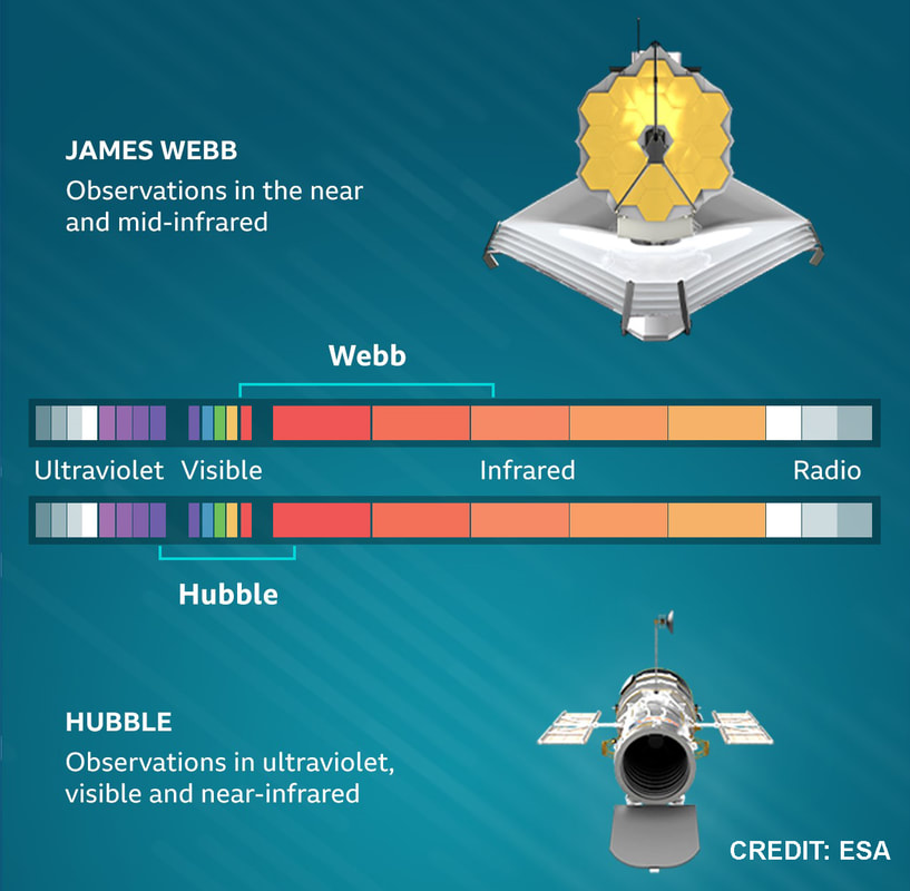 JWST vs. HST regards operating wavelength. JWST works in the near to mid infra-red bandwidth. Credit: ESA. First of all, its worth noting that it is very common for stars, in general, to possess a planetary system, and there is a large and growing catalogue of so-called exoplanets. If we think about our own planet, the depth of the atmosphere is relatively very small, being about 1.5% of the radius of the planet – and only about one tenth of this estimate corresponds to the that part of the atmosphere which is dense enough to support life. So the target of study – the atmosphere of an exoplanet – is generally very small, especially when examined remotely at such large distances. As we have mentioned in previous posts, the JWST is optimised to operate in the infra-red (IR) part of the electromagnetic spectrum, and we have discussed why this is beneficial. However, it turns out that this characteristic is also useful when investigating exoplanet atmospheres. To do this the JWST uses spectroscopy, which is simply the science of measuring the intensity of light at different wavelengths. The ‘graphical representations’ of these measurements are called spectra, and they are the key to unlocking the composition of exoplanet atmospheres. Typically, a spectrum is an array of rainbow colours, but if you capture the spectrum of, say, a star, it will also have discreet dark features called absorption lines. As the light passes through the star’s atmosphere on its way to Earth, the various elements (hydrogen, helium, etc) absorb the light at specific wavelengths, and a particular set of such lines reveals the presence of a particular element in the star’s atmosphere. 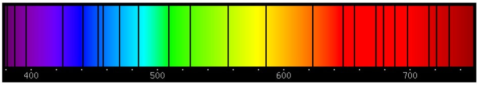 A spectrum, displaying an array of absorption lines. Credit: Source unknown. Coming back to thinking about the composition of exoplanetary atmospheres, why is IR spectroscopy such a powerful tool? It is at IR wavelengths that molecules in the atmospheres of exoplanets have the most spectral features. In particular, IR spectroscopy is especially effective in detecting molecules that are associated with life, such as water vapour, carbon dioxide, and methane. The detection of these molecules can provide evidence of habitable conditions on exoplanets and even of life itself. 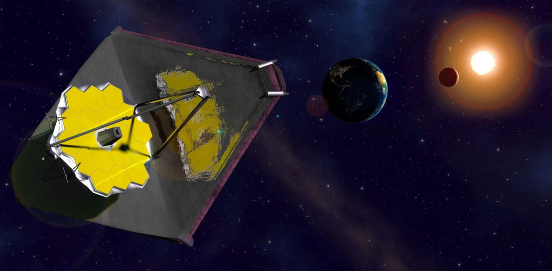 The instruments and telescope must be maintained at about -230 deg C to operate in the IR. This is achieved by keeping the telescope behind the large heat shield. Credit: Kevin Gill. So how does the JWST capture a tell-tale spectrum of the atmosphere of a distant exoplanet? The process requires that the planet transits its star at some point in the planet’s orbit. A transit occurs when the planet is between the star and the Earth, and the planet moves slowly across the disk of the star. Prior to the transit, a spectrum is taken of the star, Spectrum (star). When the planet begins its transit then the received light will have passed through the exoplanet’s atmosphere, as well as emanating from the star. A second spectrum is collected, which contains spectral features from the star and the atmosphere, Spectrum (star and planet). To acquire the spectral features of the atmosphere we difference the two, Spectrum (planet’s atmosphere) = Spectrum (star and planet) – Spectrum (star). Hopefully the accompanying diagram helps to appreciate the process. 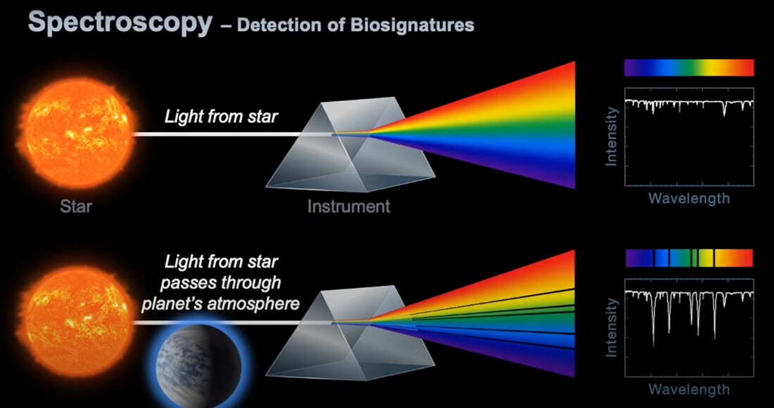 Illustration of the process of acquiring the spectrum of an exoplanet's atmosphere (note: star and planet not to scale!). Credit: Rebecca Smethurst. Getting back to the specific claims about finding evidence of life, the exoplanet concerned is designated K2-18b. The star governing this planetary system, K2-18, is to found 124 light years away in the constellation of Leo. The star is a red dwarf, which is smaller and cooler than our Sun, so that K2-18b orbits at a much closer distance than we do around our Sun. The exoplanet orbit has a radius of about 21 million km, and a period (‘year’) of 33 Earth days. This places it in the habitable zone, where it receives about the same amount of energy from its star as we receive from ours. The atmospheric composition of K2-18b was examined during two transits in January and June this year, and the results paint a picture of an ocean world with a hydrogen-dominated atmosphere. However, along with hydrogen, water vapour, carbon dioxide and methane, something else showed up called dimethyl sulphide (DMS) which caused a bit of a stir in the media. This is because the main primary and natural providers of DMS on Earth are marine bacteria and phytoplankton in our oceans. So, inevitably, it was heralded as the first detection of a ‘life signature’ on an exoplanet. 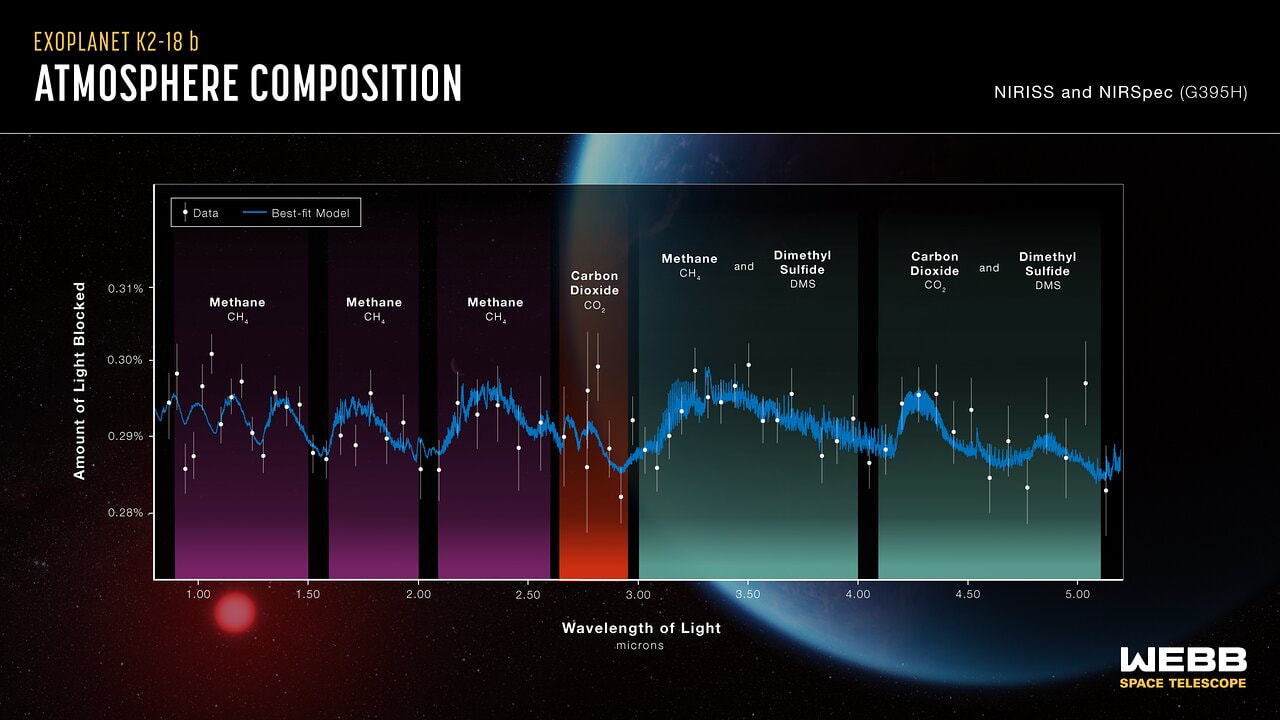 The IR spectrum of the the atmosphere of exoplanet K2-18b. Note that the vertical axis is light blocked, so that absorption features display as 'bumps'. Credit: NASA and ESA. The JWST results suggest that DMS makes up about 0.0003% of K2-18b’s atmosphere, but unfortunately in the IR bandwidth used to obtain the results, DMS is degenerate with other atmospheric species – in particular, methane and carbon dioxide. This means that the ‘bump’ in the spectrum produced by DMS is coincident with the spectral features of the other gases, so introducing a difficult ambiguity into the analysis. Looking at the results shows that there is a 1 in 60’ish chance that the detection of DMS is a statistical fluke. So, the conclusion that it is a marker for life is not secure.
Not to be put off by this, the scientists are planning more JWST observations of K2-18b using instruments that look at longer IR wavelengths where DMS absorbs more strongly and unambiguously. However, after due process, my guess is that those results will be another year or so away. I will bring you any further news as it develops … Graham Swinerd Southampton, UK October 2023 |
AuthorsJohn Bryant and Graham Swinerd comment on biology, physics and faith. Archives
July 2024
Categories |


 RSS Feed
