 Electron micrograph of a human lymphocyte. Credit: taken from hazell11bio.blogspot.com. Electron micrograph of a human lymphocyte. Credit: taken from hazell11bio.blogspot.com. John writes … Cells and organelles In order to comment on that headline, I need to start with a spot of cell biology. In all ‘eukaryotic’ organisms (i.e., all organisms except bacteria and archaea), cells contain within them several subcellular compartments or organelles. Two of these organelles, the mitochondrion (plural, mitochondria) and in plants, the chloroplast, contain a small number of genes, a reminder of their evolutionary past. These organelles were originally endosymbiotic within cells of the earliest eukaryotes. During subsequent evolution, the bulk of the endosymbionts’ genes have been taken over by the host’s main genome in the nucleus, leaving just a small proportion of their original genomes in the organelles. In mammals for example, the genes in the mitochondria make up about 0.0018 (0.18%) of the total number of genes. 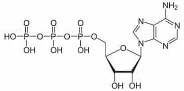 Diagram of ATP molecule. Diagram of ATP molecule. When mitochondria go wrong The main function of mitochondria is to convert the energy from food into a chemical energy currency called ATP. The average human cell makes and uses 150 million ATP molecules per day, emphasizing the absolutely key role that mitochondria play in the life of eukaryotes. This brings us back to mitochondrial genes. Although few in number, they are essential for mitochondrial function. Mutations in mitochondrial genes may lead to a lethal loss of mitochondrial function or may, in less severe cases, cause some impairment in function. During my time at the University of Exeter, I had direct contact with one such case. A very able student had elected to undertake his third-year research project with me and a colleague. However, towards the end of his second year his eyesight began to fail such that, by the start of his third year his vision was so impaired that a lab-based project was impossible. In a matter of a few months his eyesight had declined to about 15% of what he started with. The cause was a mitochondrial genetic mutation affecting the energising of the retina and hence causing impaired vision (2), a condition known as Leber hereditary optic neuropathy, symptoms of which typically appear in young adults. I need to say serious though it was for the student, this is one of milder diseases caused by mutations in a mitochondrial gene; many have much more serious effects (3), although I also need to say that diseases/syndromes based on mitochondrial genes are very rare. Is it GM or isn’t it? This brings us back to the BBC’s headline. Mitochondrial genes are only inherited from the mother. In fertilisation, the sperm delivers its full complement of nuclear genes to the egg cell but its mitochondria do not feature in the subsequent development of the embryo. In the early years of this century, scientists in several countries developed methods for replacing ‘faulty’ mitochondria in an egg cell or in a fertilised egg (one-cell embryo) with healthy mitochondria. This provides a way for a woman who knows she carries a mitochondrial mutation to avoid passing on that mutation to her offspring. However, there is another issue to deal with here. The replacement of one set of mitochondrial genes with another is clearly an example of genetic modification (GM), albeit an unusual example. In the UK, the Human Fertilisation and Embryology Act, whilst allowing spare embryos to be used in experimental procedures involving GM, prohibited the implantation of GM embryos to start a pregnancy. This would include embryos with ‘swapped’ mitochondrial DNA (or embryos derived from egg cells with swapped mitochondrial DNA). In order to bring this procedure into clinical practice, the law had to be changed which duly happened in 2015. Prior to the debates that led to the change in law, pioneers of the technique gave several presentations to explain what was involved; indeed, I was privileged to attend one of those presentations addressed to the bioscience and medical science communities. It was during this time that some opposition to the technique became apparent and the phrases ‘three-parent IVF’ and ‘three-parent babies’ became widespread both among opponents of the procedure and in the print and broadcast media.  Credit: John Bryant. Credit: John Bryant. Should we, or shouldn’t we? I will come back to the opposition in a moment but before that I want to ask whether our readers think that the use of the term ‘three-parent’ is justifiable. My friend, co-author and fellow-Christian, Linda la Velle and I discuss this on pages 52 to 54 of Introduction to Bioethics. In our view, the phrase is inaccurate and misleading and I was pleased to see that the recent BBC headline (in the title of this post) did not use it, even if the headline still conveyed slightly the wrong impression.  ‘Designer baby’. Credit: taken from www.makeuseof.com. ‘Designer baby’. Credit: taken from www.makeuseof.com. Returning to consider the opposition to the technique, there were some who believed that allowing it would open the gate to wider use of GM techniques with human embryos, leading to the possibility of ‘designer babies’. However, there were other reasons for opposition. Since its inception with the birth of Louise Brown in 1978, IVF has had its opponents who believe that it debases the moral status of the human embryo. According to their view, which I need to say, is not widely held (4), the one-cell human embryo should be granted the same moral status as a born human person, from the ‘moment of conception’. There can be no ‘spare’ embryos because that would be like saying there are spare people. This brings us to the two different techniques described in the recent BBC article. 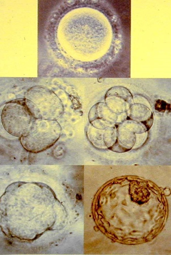 The first few days of growth of a human embryo produced by IVF. The one-cell embryo, subject of one of the techniques for swapping mitochondria, is at the top. It is about 0.15 mm in diameter. Credit: Source unknown. How is it done? As hinted at briefly already, there are two methods for removing faulty mitochondria and replacing them with fully functioning mitochondria, as shown in the HFEA diagram (below) reproduced by the BBC. In passing, I note that the ability to carry out these techniques owes a lot to what was learned during the development of mammalian cloning. In the first technique, an egg (5) is donated by a woman who has normal mitochondria. This egg is fertilised by IVF as is an egg from the prospective mother who is at risk of passing on faulty mitochondria. We now have two fertilised eggs/one-cell embryos. The nucleus (which contains most of the genes) is removed from the embryos derived from the donated egg and is replaced with the nucleus from the embryo with faulty mitochondria. Thus nuclear transfer has been achieved, setting up a ‘hybrid’ embryo (nucleus from the embryo with faulty mitochondria, ‘good’ mitochondria in the embryo derived from the donated egg). The embryo can then be grown on for two or three days before implantation into the prospective mother’s uterus, hopefully to start a pregnancy. However, readers will immediately realise that this method effectively involves destruction of a human one-cell embryo, raising again objections from those who hold the view that the early embryo has the same moral status as a person (see above). 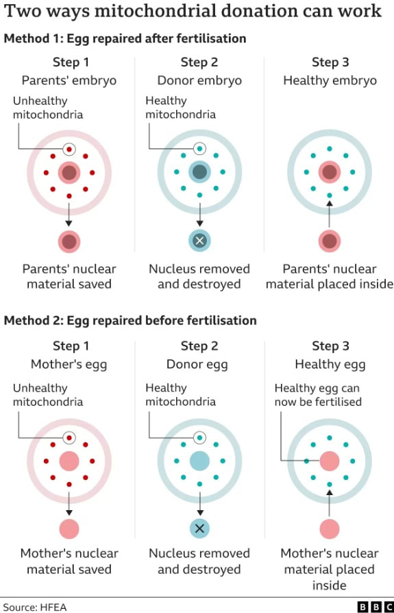 Diagrams of the two methods for swapping mitochondria. Credit: HFEA This brings us to the second method. It again involves donation of an egg with healthy mitochondria but this is enucleated without being fertilised. Nuclear transfer from an egg of the prospective mother with faulty mitochondria then creates a ‘hybrid’ egg which is only then fertilised by IVF and cultured for a few days prior to implantation into the uterus of the prospective mother. The technique does not inherently involve destruction of a one-cell human embryo. However, since the procedure, including IVF, will be carried out with several eggs, there still remains the question of spare embryos, mentioned above. Further, since this technique leads to less success in establishing pregnancies than the first technique, it is likely not to be the technique of first choice in these situations. So when was that, exactly? The BBC report which stimulated me to write this blog talked of a ‘UK First’ but that cannot mean that the world’s first case was in the UK. There are well-documented reports from at least three different countries and going back to 2016, of babies born following use of nuclear transfer techniques. The headline must imply that this was the first case in the UK. However, following the change in the law (mentioned above), in 2017 the Human Fertilisation and Embryology Authority (HFEA) licensed the Newcastle Fertility Centre to carry out this procedure. It was predicted that the first nuclear transfer/mitochondrial donation baby would be born in 2018 (although we emphasise that because of the rarity of these mitochondrial gene disorders the number of births achieved by this route will be small). So, when was the first such baby actually born in the UK. The answer is that we do not know. The HFEA, which regulates the procedure, is very protective of patient anonymity and does not release specific information that might identify patients. All we know is that ‘fewer than five’ nuclear transfer/mitochondrial donation babies have been born and that the births have taken place between 2018 and early 2023 – so, in respect of the date of this ‘UK First’ we are none the wiser. John Bryant
Topsham, Devon 28 June 2023 (1) Baby born from three people’s DNA – BBC News. (2) My colleague and I were able to offer him a computer-based project and the university’s special needs office provided all that he needed to complete his degree. (3) See, for example: Mitochondrial DNA Common Mutation Syndromes, Children’s Hospital of Philadelphia – chop.edu. (4) In Life in Our Hands (IVP, 2004) and Beyond Human? (Lion Hudson, 2012), I discuss the wide range of views on this topic among Christians. (5) Although I use the singular for the sake of convenience, several donated and several maternal eggs are used in these procedures.
0 Comments
Graham writes … This question has occupied cosmologists since the theory of cosmic inflation was first developed by Alan Guth in 1979, who realised that empty space could provide a mechanism to account for the expansion of the Universe. 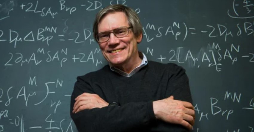 Alan Guth has been dubbed the father of cosmic inflation theory. Credit: Deanne Fitzmaurice / National Geographic Image Collection / Alamy. In the theory it is assumed that a tiny volume of space-time in the early Universe – very much smaller than a proton – came to be in a ‘false vacuum’ state. Effectively, in this state space is permeated by a large, constant energy density. The effect of this so-called ‘inflaton field’ is to drive a rapid expansion of space-time for as long as the false vacuum state exists. I won’t go into the detail of how this happens here (1), but as a consequence the tiny nugget of space-time grows exponentially, before the energy density decays to acquire a ‘true vacuum’ state once again, bringing the inflationary period to an end. Theoretically, this expansion takes place between roughly 10 to the power -36 (10e-36) sec (2) and 10e-32 sec after the bang (ATB) – periods of time that makes the blink of an eye seem like an eternity. To generate a universe with the characteristics we observe today, the expansion factor must be of the order of 10e+30. To give an impression of what this degree of expansion means, if you expand a human egg cell by a factor of 10e+25, you get something about the size of the Milky Way galaxy! The diagram below helps, I think, to illustrate the time line of developments ATB. Clearly the horizontal time axis is not linear! 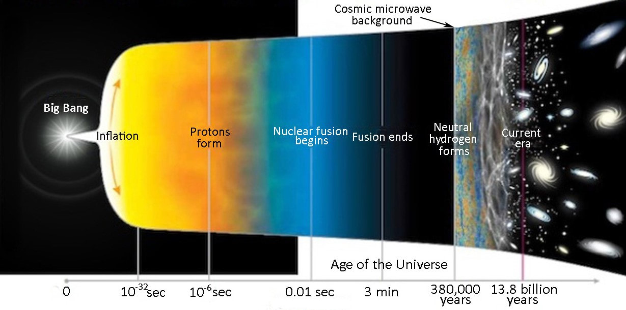 Timeline of significant events in the evolution of the Universe. Credit: Source unknown. 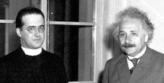 Georges Lemaître (left) with Albert Einstein. Lemaître was a Belgium priest and physicist. Credit: public domain. Georges Lemaître (left) with Albert Einstein. Lemaître was a Belgium priest and physicist. Credit: public domain. To me, the events of the inflation era seem extraordinary, prompting the question in the title of this post. However unlikely these events may seem, the cosmic inflation paradigm has been very successful in resolving problems which have dogged the ‘conventional’ theory of the big bang as originally proposed by Georges Lemaître in 1927 (3), for example, the horizon and flatness problems. A summary of these issues, and others, can be found here. When we use Einstein’s field equations of general relativity, we make an assumption that on cosmic scales of billions of light years, the Universe is homogeneous and isotropic. In other words, it appears the same at all locations and in all directions. These simplifying symmetries are what allows us to use the mathematics to study the large-scale dynamics of the Universe. A nice analogy is to think of the Universe as a glass of water, and each entire galaxy as a molecule of H2O. In using the equations, we are examining the glass of water, and ignoring the small-scale molecules. However, cosmology at some point has to come to terms with the idea that when you examine the Universe at smaller scales you find clumpy structures like galaxies. And here we are faced with a conundrum. 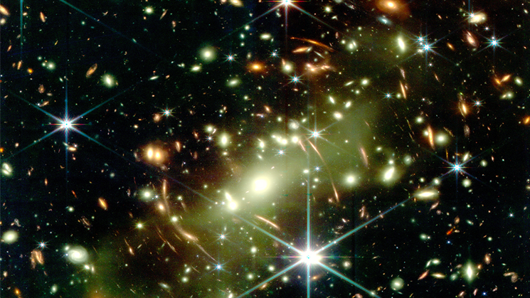 A beautiful array of 'clumpy structures' displayed in this JWST deep field image. Credit: Aaron Robotham (ICRAR-UWA). The primary question addressed in this post is along the lines of ‘what is the origin of the inhomogeneities that led to the development of the clumpy structures like galaxies and stars that we observe today?’ Without these, clearly we would not be here to contemplate the issue. If we assume that cosmic inflation occurred, then the initial ‘fireball’ would be microscopically tiny. Its extreme temperature and energy density, just ATB but before the inflationary expansion, would be able to reach equilibrium smoothing out any variations. So, the question posed above becomes key. If the resulting density and temperature of the inflated universe was uniform, then how did galaxies form? Where did the necessary inhomogeneities come from? It is gratifying that the inflation theory offers progress in answering this question – indeed, remarkably, the initial non-uniformities that gave rise to galaxies and stars may have come from quantum mechanics! 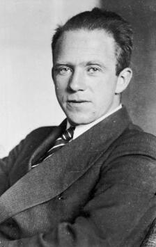 Werner Heisenberg. Credit: Bundesarchiv / public domain. Werner Heisenberg. Credit: Bundesarchiv / public domain. This magnificent idea arises from the interplay between inflationary expansion and the quantum uncertainty principle. The uncertainty principle, originally proposed by Werner Heisenberg, says that there are always trade-offs in how precisely complementary physical quantities can be determined. The example most often quoted involves the position and speed of a sub-atomic particle. The more precisely its position is determined, the less precisely it speed can be determined (and the other way round). However, the principle can also be applied to fields. In this case, the more accurate the value of a field is determined, the less precisely the field’s rate of change can be established, at a given location. Hence, if the field’s rate of change cannot be precisely defined, then we are unable to determine the field’s value at a later (or earlier) time. At these microscopic scales the field’s value will undulate up or down at this or that rate. This results in the observed behaviour of quantum fields – their value undergoes a characteristic frenzied, random jitter, a characteristic often referred to as quantum fluctuations. This takes us back then to the inflaton field that drives the dramatic inflationary expansion of the early Universe. In the discussion in the book (1), as the inflationary era is drawing to a close it is assumed that the energy of the field decreased and arrived at the true vacuum state at the same time at each location. However, the quantum fluctuations of the field’s value means that it reaches its the value of lowest energy at different places at slightly different times. Consequently, inflationary expansion shuts down at different locations at different moments, resulting in differing degrees of expansion at each location, giving rise to inhomogeneities. Hence, inflationary cosmology provides a natural mechanism for understanding how the small-scale nonuniformity responsible for clumpy structures like galaxies emerge in a Universe that on the largest scales is comprehensively homogeneous. 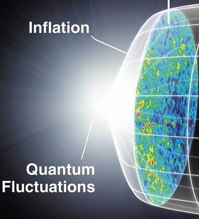 The cosmic microwave background was created at around 380,000 years ATB. 3D space is represented here as a 2D disk imprinted with temperature fluctuations. Credit: Source unknown. The cosmic microwave background was created at around 380,000 years ATB. 3D space is represented here as a 2D disk imprinted with temperature fluctuations. Credit: Source unknown. So quantum fluctuations in the very early Universe, magnified to cosmic size by inflation, become the seeds for the growth of structure in the Universe! But is all this just theoretical speculation, or can these early seeds be observed? The answer to this question is very much ‘yes!’. In 1964 two radio astronomers, Arno Penzias and Robert Wilson made a breakthrough discovery (serendipitously). The two radio astronomers detected a source of low energy radio noise spread uniformly across the sky, which they later realised was the afterglow of the Big Bang. This radiation, which became know as the cosmic microwave background (CMB), is essentially an imprint of the state of the Universe at around 380,000 years ATB (4). Initially the Universe was a tiny, but unimaginably hot and dense ‘fireball’, in which the constituents of ‘normal matter’ – protons, neutrons and electrons – were spawned. Initially electromagnetic (EM) radiation was scattered by its interaction with the charged particles so that the Universe was opaque. However, when the temperature decreased to about 3,000 degrees Celsius, atoms of neutral hydrogen were able to form, and the fog cleared. At this epoch, the EM radiation was released to propagate freely throughout the Universe. Since that time the Universe has expanded by a factor of about one thousand so that the radiation’s wavelength has correspondingly stretched, bringing it into the microwave part of the EM spectrum. It is this remnant radiation that we now call the CMB. It is no longer intensely hot, but now has an extremely low temperature of around 2.72 Kelvin (5). This radiation temperature is uniform across the sky, but there are small variations – in one part of the sky it may be 2.7249 Kelvin and at another 2.7251 Kelvin. So the radiation temperature is essentially uniform (the researchers call it isotropic), but with small variations as predicted by inflationary cosmology. 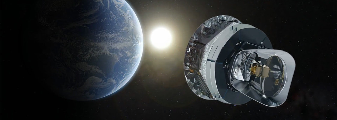 The European Space Agency's Planck mission has produced the most accurate thermal map of the cosmic microwave background. Credit: ESA. 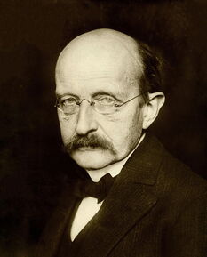 Max Planck. Credit: public domain. Max Planck. Credit: public domain. Maps of the temperature variations in the CMB have been made by a number of satellite missions with increasing accuracy. The most recent and most accurate was acquired by ESA’s Planck probe, named in honour of Max Planck, one of the pioneering scientists that developed the theory of quantum mechanics. The diagram below displays the primary results of the Planck mission, showing a colour coded map of the CMB temperature fluctuations across the sky. Note that these variations are small, amounting to differences at the millidegree level (6). This map may not look very impressive to the untrained eye, but it represents a treasure trove of information and data about the early Universe which has transformed cosmology from the theoretical science it used to be to a science based on a foundation of observational data. 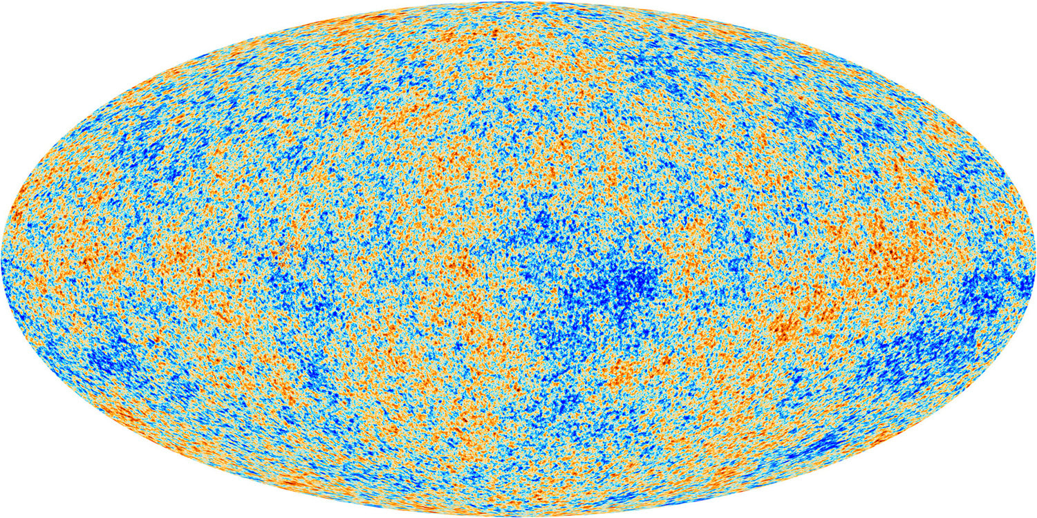 The tiny temperature variations in the CMB across the sky derived from the Planck spacecraft mission. Credit: ESA. The final icing on the cake is what happens when you carry out calculations based on the predictions of quantum mechanics that we discussed earlier. The details are not important here, but diagram 1 shows the prediction where the horizontal axis shows the angular separation of two points on the sky, and the vertical axis shows their temperature difference. In diagram 2 this prediction is compared with satellite observations and as you can see there is remarkable agreement! 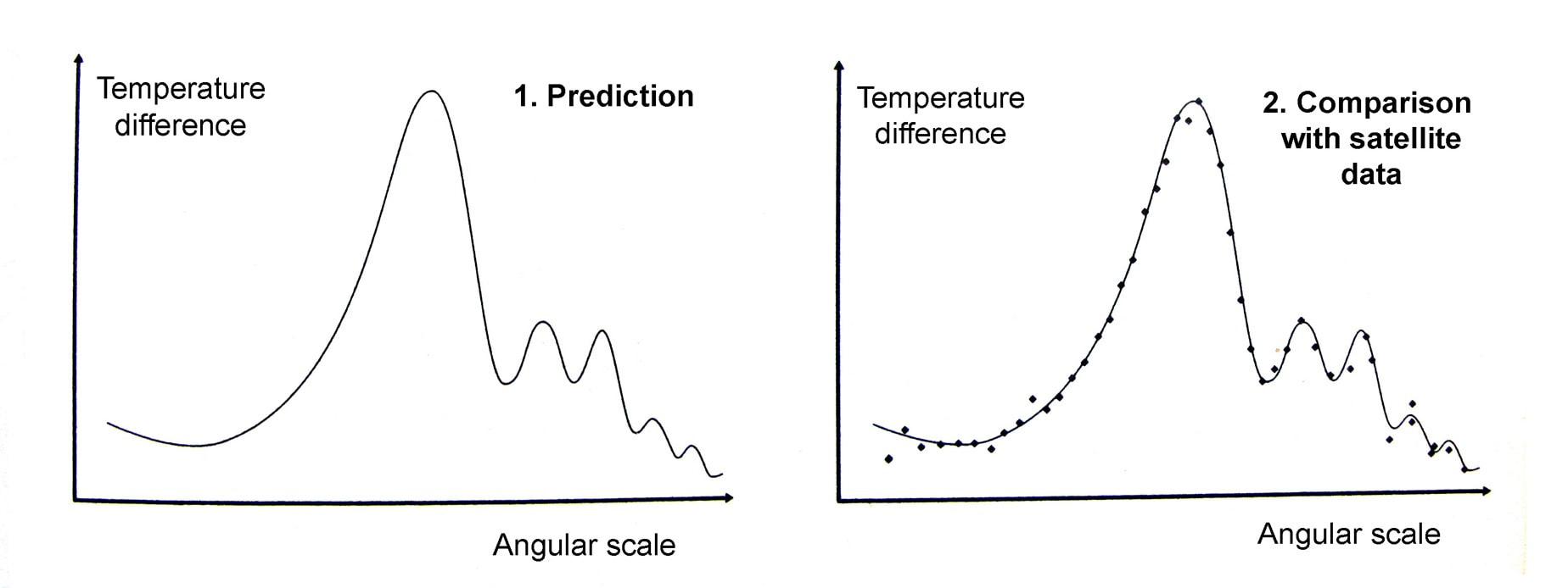 Comparison of theory (1) with satellite data (2). Data points in (2) are probably those obtained by the earlier COBE (Cosmic Background Explorer) mission. Credit: Brian Greene / reference (7). This success has convinced many physicists of the validity of inflationary cosmology, but many remain to be convinced. Despite the remarkable success of the theory, the associated events that occurred 13.8 billion years ago seem to me to be extraordinary. And then, of course, there is also the issue of the origin and characteristics of the inflaton field that kicked it all off.
Despite all this, however, I am blown away by the notion that the 100 billion or more galaxies in our visible Universe may be ‘nothing but quantum mechanics writ large across the sky’, to quote Brian Greene (7) Graham Swinerd Southampton, UK May 2023 (1) Graham Swinerd and John Bryant, From the Big Bang to Biology – where is God?, Kindle Direct Publishing, 2020, see Section 3.6 for more detail. (2) In the website editor, I am unable to use the usual convention of employing superscripts to represent ‘10 to the power of 30’ for example. In the text I have used the notation 10e+30 to denote this. (3) Georges Lemaître’s publication of 1927 appeared in a little-known Belgium journal. It was subsequently published in 1931 in a journal of the Royal Astronomical Society. (4) Graham Swinerd and John Bryant, From the Big Bang to Biology: where is God?, Kindle Direct Publishing, 2020, pp. 60 – 63 for more details about the CMB. (5) The Kelvin temperature scale is identical to the Celsius scale but with zero Kelvin at absolute zero (-273 degrees Celsius). Hence, for example, water freezes at +273 Kelvin and boils at +373 Kelvin. (6) A millidegree is 1 thousandths of a degree. (7) Brian Green, The Fabric of the Cosmos, Penguin Books, 2004, pp. 308-309.  John writes … ‘Cardiff scientists look at honey as drug alternative’ (1) – a headline that intrigued both me and Dave Piper of Trans World Radio (TWR-UK), leading to his request to interview me about it (2). On the surface it seems rather strange or even crazy but there are good reasons why it may not be as strange as it appears. I will return to this later but first I want to look more generally at our dependence on plants for important pharmaceuticals. The World Health Organisation (WHO) publishes a long list of Essential Medicines, last updated in 2021 (3); over 100 of them were first derived from or are still extracted from flowering plants, including the examples I discuss below. In the immortal words of Michael Caine ‘Not a lot of people know that’. Over the millennia of human existence, people have turned to the natural world for help in combatting a wide range of ailments from everyday aches and pains to serious illnesses. Many of these folk remedies were not, as we would now say, ‘evidence-based’: they did not actually work. Equally however, many have now been shown to point to the existence of genuinely therapeutic chemicals, as shown by four examples. I have discussed them in some detail because I really want our readers to understand how dependent we are on the natural biodiversity of the plant kingdom – a feature that is constantly under threat.  Willow. Willow. Aspirin. Accounts of the use of extracts of willow (Salix) leaves and bark to relieve pain and to treat fevers occur as far back as 2,500 BCE, as evidenced by inscriptions on stone tablets from the Sumerian period. Willow bark was also used by the ancient Egyptians while Hippocrates (460-377 BCE) recommended an extract of willow bark for fever, pain and child-birth. The key chemical in willow has the common name of salicin, first purified in the early 19th century. In the human body, this is metabolised to salicylic acid which is the bioactive compound that has the medicinal effects. Meadowsweet (Spirea ulmaria) leaves also contain salicin and the medicinal properties of this plant had led in earlier centuries to the Druidic Celts regarding it as sacred.  Salicylic acid was synthesised in the lab for the first time in 1859 and the pure form was used with patients shortly after that. Unfortunately, the acid has a very unpleasant taste and also irritates the stomach so is not ideal for use as a regular medication. However, in 1897, a team led by Dr Felix Hoffman at Friedrich Bayer and Co. in Germany managed to synthesise a derivative, acetyl-salicylic acid which has a less nasty taste and is much less of an irritant than the parent compound. After successful clinical trials, the compound was registered as aspirin in 1899. This was the first drug to be made synthetically and the event is regarded as the birth of the pharmaceutical industry. Interestingly, the place of acetyl-salicylic acid in the WHO list is based, not on its pain-killing properties but on its action as a blood-thinner. Morphine. Morphine is a powerful narcotic and pain killer that is synthesised by the opium poppy (Papaver somniferum); extracts of the plant, known as opium, have been used medicinally and recreationally for several thousand years, both in Europe and in what we now call the Middle East. Indeed, as long ago as 4,000 BCE in Mesopotamia, the poppy was called the ‘plant of joy.’ In Europe, the medicinal use of opium, often as a tincture or as a solution in alcohol was popularised from the 16th century onwards. In addition, the seeds or extracts of seeds, often in the form of a poppy seed cake or mixed with milk or honey have been given to babies and small children to help them sleep (4) (the Latin name of the plant means sleep-inducing poppy).  Opium poppy. Credit: Louise Joly via Wikipedia Commons. Opium poppy. Credit: Louise Joly via Wikipedia Commons. The active ingredient of opium is morphine which was first isolated by a German pharmacist, Freidrich Sertürner in 1803. It was thus the first medicinally active ingredient to be isolated from a plant (as opposed to salicylic acid – see above – which was the first to be chemically synthesised). It was originally called morphium, after the Greek god of dreams, Morpheus but the name was changed to morphine when Merck started to market it in 1827. Over the past 15 years methods have been developed for its chemical synthesis but none of these are as yet anything like efficient enough to meet the demand for the drug and so it is still extracted from plant itself. 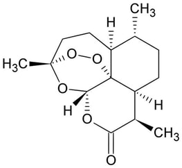 Structure of Artemisinin: Public Domain. Structure of Artemisinin: Public Domain. Artemisinin. In China, extracts of the sweet wormwood plant (Artemisia annua) have been used to treat malaria for about 2,000 years. The active ingredient was identified as an unusual and somewhat complex sesquiterpene lactone (illustrated, for those with a love of organic chemistry!) which was named artemisinin. It was added to the WHO list after extensive clinical trials in the late 20th century. Artemisinin has not been chemically synthesised ‘from scratch’ and initial efforts to increase production involved attempts to breed high-yielding strains of A. annua. However, it proved more efficient to transfer the relevant genes into the bacterium Escherichia coli or yeast cells, both of which can be grown on an industrial scale (5). The genetically modified cells synthesise artemisinic acid which is easily converted into artemisinin in a simple one-step chemical process.  Rosy Periwinkle. Credit: Royal Botanic Gardens, Kew via Creative Commons. Rosy Periwinkle. Credit: Royal Botanic Gardens, Kew via Creative Commons. Vinblastine and Vincristine. These two anti-cancer drugs were isolated from leaves of the Madagascar periwinkle (6) (which is not actually confined to Madagascar). The original Latin name for this plant was Vinca rosea (hence the names of the two drugs) but is now Catharanthus roseus. In Madagascar, a tea made with the leaves had been used as a folk remedy for diabetes and the drug company, Eli Lilly took an interest in the plant because of this. However, controlled trials in the late 1950s and early 1960s gave, at best, ambiguous results and no anti-diabetic compounds were found in leaf extracts. However, the company did detect a compound that prevented chromosomes from separating and thus inhibited cell division. The compound was named vincristine. Further, a research team at the University of Western Ontario discovered a similar compound with similar inhibitory properties; this was named vinblastine. Because the two compounds inhibit cell division, they were trialled as anti-cancer drugs and are now part of an array of pharmaceuticals which may be used in chemotherapy (7). In past 15 years, both have been chemically synthesised from simple precursors but we still rely on extraction form plants for the bulk of the required supply. I also want to emphasise that these are far from being the only anti-cancer drugs derived from plants, discussed by Dr Melanie-Jayne Howes of the Royal Botanic Gardens, Kew (8). As she says, plants are far better at synthetic chemistry than humans! Back to the beginning. In the book we describe the natural world as a network of networks of interacting organisms. Given that context, we need to think about the natural function of these compounds that humans make use of in medicine. A brief overview suggests that many of them have a protective role in the plant. This may be protection against predators or disease agents or against the effects of non-biological stresses. Thinking about the former brings us back to the topic that I started with, namely looking for ‘drug alternatives’. The story starts with another interaction, namely that the fungus Penicillium notatum synthesises a compound that inhibits the growth and reproduction of bacteria; that compound was named penicillin and was the first antibiotic to be discovered (in 1928). However, as with the examples of drugs from plants mentioned earlier, we see hints of the existence of anti-biotics in ancient medical practices. In China, Egypt and southern Europe, mouldy bread had been used since pre-Christian times to prevent infection of wounds and the practice of using ‘moulds’ (probably species of Penicillium or Rhizopus) to treat infections was documented in the early 17th century by apothecary/herbalist/botanist John Parkinson who went on to be appointed as Apothecary to King James I. It is not just plants that supply us with essential drugs: the fungus kingdom also comes up with the goods. Antibiotics are a subset of the wider class of anti-microbials, chemicals that are effective against different types of micro-organisms, including micro-fungi, protists and viruses. Artemisinin, mentioned above, is thus an anti-microbial. Many anti-microbials are – or were initially – derived from natural sources while others have been synthesised by design to target particular features of particular micro-organisms. There is no doubt that their use has saved millions of lives. However, we now have a major problem. The over-use of antibiotics and other anti-microbials in medicine, in veterinary medicine and in agricultural animal husbandry has accelerated the evolution of drug-resistant micro-organisms against which anti-microbials are ineffective. The WHO considers this to be a major threat to our ability to control infectious diseases and hence there is a widespread search for new anti-microbials. The search is mainly focussed on the natural world although there are some attempts to design drugs from scratch using sophisticated synthetic chemistry. The Cardiff team who headlined this article are looking at plants and at products derived from plants. The ‘drug alternatives’ mentioned in the BBC headline refer to the team’s hopes of finding new anti-microbials. They have noted that in earlier centuries, honey had been used in treating and preventing infection of wounds and they wonder whether it contains some sort of anti-microbial compound. The plants that have contributed to a batch of honey can be identified by DNA profiling of any cellular material, especially pollen grains, in the honey. The team is especially interested in honey derived or mainly derived from dandelion nectar because dandelions synthesise a range of protective chemicals and in herbal medicine are regarded as having health-giving properties. So … the hunt is on and we look forward to hearing more news from Cardiff in due course.  John Bryant
Topsham, Devon April 2023 All images by John Bryant, except those credited otherwise. (1) Cardiff scientists look at honey as drug alternative – BBC News. (2) www.youtube.com. (3) World Health Organisation model list of essential medicines – 22nd list, 2021. (4) This was certainly practised in parts of central Europe in the mid-20th century. (5) See J. A. Bryant & L. La Velle, Introduction to Bioethics (2nd edition), Wiley, 2018, p. 200. (6) See J.A. Bryant & L. La Velle, Introduction to Bioethics (2nd edition), Wiley, 2018, pp. 241-242. (7) Interestingly, a recent paper claims that traditional Indian medicine has made use of the anti-tumour properties of C. roseus: Mishra & Verma, International Journal of Research in Pharmacy and Pharmaceutical Sciences, 2017, Vol. 2, pp. 20-23. (8) Plants and the evolution of anticancer drugs – Royal Botanic Gardens Kew. 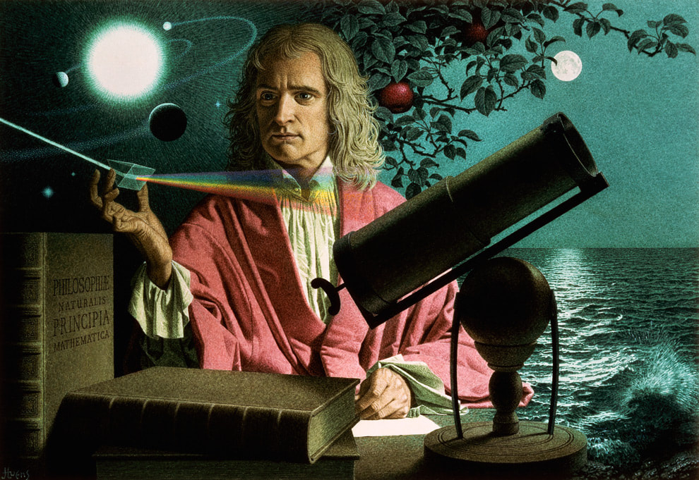 Portrait of Sir Isaac Newton by Jean-Leon Huens. Credit Jean-Leon Huens National Geographic Stock Graham writes … Isaac Newton was the first to really appreciate the concept that mathematics has the power to reveal deep truths about the physical reality in which we live. Combining his laws of motion and gravity, he was able to construct equations which he could solve having also developed the basic rules of what we now call calculus (1). A remarkable individual achievement, which unified a number of different phenomena – for example, the fall of an apple, the motion of the moon, the dynamics of the solar system – under the umbrella of one theory. 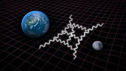 Unification of gravity and the quantum still evades resolution. Credit SLAC National Accelerator Lab Unification of gravity and the quantum still evades resolution. Credit SLAC National Accelerator Lab Coming up to the present day, this pursuit of unification continues. In summary, the objective now is to find a theory of everything (TOE), which is something that has occupied the physics community since the development of the quantum and relativity theories in the early 20th century. Of course, the task now is somewhat more challenging than that of Newton. He had ‘simply’ gravity to contend with, whereas now, physicists have so far discovered four fundamental forces – gravity, electromagnetism, the weak and strong nuclear forces – which govern the way the world works. Along the way in all this, we have accumulated a significant understanding of the Universe, both on a macroscopic scale (astrophysics, cosmology) and on a micro scale (quantum physics).  Why do the laws of physics appear to be 'bio-friendly'? Credit: Source unknown. Why do the laws of physics appear to be 'bio-friendly'? Credit: Source unknown. One surprising consequence of all this, is that we have discovered that the Universe is a very unlikely place. So, what do I mean by this? The natural laws of physics and the values of the many fundamental constants that specify how these laws work appear to be tuned so that the Universe is bio-friendly. In other words, if we change the value of just one of the constants by a small amount, something invariably goes wrong, and the resulting universe is devoid of life. The extraordinary thing about this tuning process is just how finely-tuned it is. American physicist Lee Smolin (2) claims to have quantitatively determined the degree to which the cosmos is finely tuned when he says: “One can estimate the probability that the constants in our standard theories of the elementary particles and cosmology would, were they chosen randomly, lead to a world with carbon chemistry. That probability is less than one part in 10 to the power 220.” The reason why this is so significant for me, is that this characteristic of the Universe started me on a personal journey to faith some 20 years ago. Clearly, in itself, the fine-tuning argument does not prove that there is (or is not) a God, but for me it was a strong pointer to the idea that there may be a guiding intelligence behind it all. At that time, I had no religious propensities at all and the idea of a creator God was anathema to me, but even I could appreciate the significance of the argument without the help of Lee Smolin’s mysterious calculations. This was just the beginning of a journey for me, which ultimately led to a spiritual encounter. At the time, this was very unwelcome, as I had always believed that the only reality was physical. However, God had other ideas, and a belief in a spiritual realm has changed my life. However, that is another story, which I tell in some detail in the book if you are interested (3). The purpose of this blog post is to pose a question. When we look at the world around us, and at the Universe at macro and micro scales, we can ask: did it all happen by blind chance, or is there a guiding hand – a source of information and intelligence (“the Word”) – behind it all? There are a number of thought-provoking and intriguing examples of fine-tuning discussed in the book (3), but here I would like to consider a couple of topics not mentioned there, both of which focus on the micro scale of quantum physics.  If the protons and neutrons in this picture were 10 cm in diameter, then the quarks and electrons would be less than 0.1 mm in size and the entire atom would be about 10 km across. Credit: Source unknown. If the protons and neutrons in this picture were 10 cm in diameter, then the quarks and electrons would be less than 0.1 mm in size and the entire atom would be about 10 km across. Credit: Source unknown.
There is general agreement among physicists that something extraordinary occurred then, which in the standard model of cosmology is called the ‘Big Bang’ (BB). There is debate as to whether this was the beginning of our Universe, when space, time, matter and energy, came into existence. Some punters have proposed other scenarios; that perhaps the BB marked the end of one universe and the beginning of another (ours), or that perhaps the ‘seed’ of our Universe had existed in a long-lived quiescent state until some quantum fluctuation had kicked off a powerful expansion – the possibilities are endless. But one thing we do know about 13.8 billion years ago is that the Universe then was very much smaller than it is now, unimaginably dense and ultra-hot. The evidence for this is incontrovertible, in the form of detailed observations of the cosmic microwave background (4). If we adopt the standard model, the events at time zero are still a mystery as we do not have a TOE to say anything about them. However, within a billionth of a billionth of a billionth of second after the BB, repulsive gravity stretched a tiny nugget of space-time by a huge factor – perhaps 10 to the power 30. This period of inflation (5) however was unstable, and lasted only a similarly-fleeting period of time. The energy of the field that created the expansion was dumped into the expanding space and transformed (through the mass-energy equivalence) into a soup of matter particles. It is noteworthy that we are not sure what kind of particles they were, but we do know that, at this stage of the process, they were not the ‘familiar’ ones that make up the atoms in our body. After a period of a few minutes, during which a cascade of rapid particle interactions took place throughout the embryonic cosmos, a population of protons, neutrons and electrons emerged. In these early minutes of the universe, the energy of electromagnetic radiation dominated the interactions and the expansion dynamics, disrupting the assembly of atoms. However, thereafter, there was a brief window of opportunity when the Universe was cool enough for this disruption to cease, but still hot enough for nuclear reactions to take place. During this interval, a population of about 76% hydrogen and 24% helium resulted, with a smattering of lithium (6). In all this, an important feature is the formation of stable proton and neutron particles, without which, of course, there would be no prospect of the development of stars, galaxies and, ultimately, us. To ‘manufacture’ a proton, for example, you need two ‘up’ quarks and one ‘down’ quark (to give a positive electric charge), stably and precisely confined within a tiny volume of space by a system of eight gluons. Without dwelling on the details, the gluons are the strong force carriers which operate between the quarks using a system of three different types of force (arbitrarily labelled by three colours). Far from being a fundamental particle, the proton is comprised of 11 separate particles. The association of quarks and gluons is so stable (and complex) that quarks are never observed in isolation. Similarly, neutrons comprise 11 particles with similar characteristics, apart from there being one ‘up’ quark and two ‘down’ quarks, to ensure a zero electric charge. So what are we to say about all this? Is it likely that all this came about by blind chance? Clearly, the processes I have described is governed by complex rules – the laws of nature – to produce the Universe that we observe. So, in some sense the laws were already ‘imprinted’ on the fabric of space-time at or near time zero. But in the extremely brief fractions of a second after the BB where did they come from? Who or what is the law giver? Rhetorical questions all, but there are a lot of such questions in this post to highlight the notion that such complex behaviour (order) is unlikely to occur simply by ‘blind chance’. 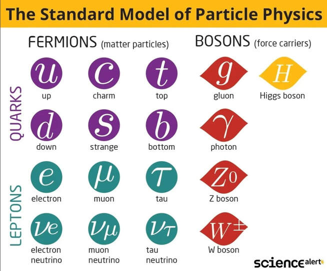
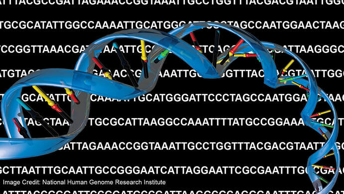
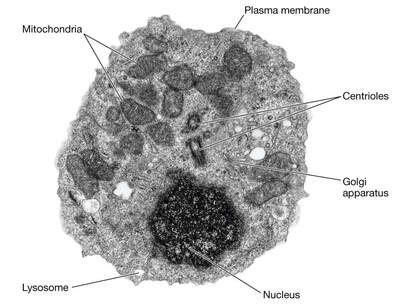
There have been many ‘eureca moments’ in physics, when suddenly things fall into place and order is revealed. One such situation arose in the 1950s, when the increasing power of particle colliders was generating discoveries of many new particles. So many in fact that the physics community was running out of labels for the members of this growing population. Then in 1961, a physicist named Murray Gell-Mann came up with a scheme based upon a branch of mathematics called group theory which made sense of the apparent chaos. His insight was that all the newly discovered entities were made of a few smaller, fundamental particles that he called ‘quarks’. As we have seen above, protons and neutrons comprise three quarks, and mesons, for example, are made up of two. Over time this has evolved into something we now refer to as the standard model of particle physics, which consists of 6 quarks, 6 leptons, 4 force carrier particles and the Higgs boson, as can be seen in the diagram (the model also includes each particle’s corresponding antiparticle). These particles are considered to be fundamental – that is, they are indivisible. We have talked about this in a couple of previous blog posts – in October 2021 and March 2022 – and it might be worth having a look back at these to refresh your memory. Also, as we have seen before, we know that the standard model is not perfect or complete. Gravity’s force carrier, the graviton, is missing, as are any potential particles associated with the mysterious dark universe – dark matter and dark energy. Furthermore, there is an indication of missing constituents in the model, highlighted by the recent anomalous experimental results describing the muon’s magnetic moment (see March 2022 post). I have recently been reading a book (7) by physicist and author Paul Davies, and, although his writings are purely secular, I think my desire to write on today’s topic has been inspired by Davies’s thoughts on many philosophical conundrums found there. The fact that the two examples I have discussed above have an underlying mathematical structure that we can comprehend is striking. Furthermore, there are many profound examples of this structure leading to successful predictions of physical phenomena, such as antimatter (1932), the Higgs Boson (2012) and gravitational waves (2015). Davies expresses a view that if we can extract sense from nature, then it must be that nature itself is imbued with ‘sense’ in some way. There is no reason why nature should display this mathematical structure, and certainly no reason why we should be able to comprehend it. Would processes that arose by ‘blind chance’ be underpinned by a mathematical, predictive structure? – I’m afraid, another question left hanging in the air! I leave the last sentiments to Paul Davies, as I cannot express them in any better way. “How has this come about? How have human beings become privy to nature’s subtle and elegant scheme? Somehow the Universe has engineered, not just its own awareness, but its own comprehension. Mindless, blundering atoms have conspired to spawn beings who are able not merely to watch the show, but to unravel the plot, to engage with the totality of the cosmos and the silent mathematical tune to which it dances.” Graham Swinerd Southampton March 2023 (1) Graham Swinerd and John Bryant, From the Big Bang to Biology: where is God?, Kindle Direct Publishing, 2020, Chapter 2. (2) Lee Smolin, Three Roads to Quantum Gravity, Basics Books, 2001, p. 201. (3) Graham Swinerd and John Bryant, From the Big Bang to Biology: where is God?, Kindle Direct Publishing, 2020, Chapter 4. (4) Ibid., pp. 60-62. (5) Ibid., pp. 67-71. (6) Ibid., primordial nucleosynthesis, p.62. (7) Paul Davies, What’s Eating the Universe? and other cosmic questions, Penguin Books, 2021, p. 158.  Donald Pleasance plays Blofeld in You Only Live Twice. Credit: E! News. John writes … As we have written in the book, one of the essential requirements for life is an information-carrying molecule that can be replicated/self-replicated. That molecule is DNA, the properties and structure of which fit it absolutely beautifully for its job. That DNA is the ‘genetic material’ seems to be embedded in our ‘folk knowledge’ but it may surprise some to know that the unequivocal demonstration of DNA’s role was only achieved in the mid-1940s. This was followed nine years later by the elucidation of its structure (the double helix), leading to an explosion of research on the way that DNA actually works, how it is regulated and how it is organised in the cell. 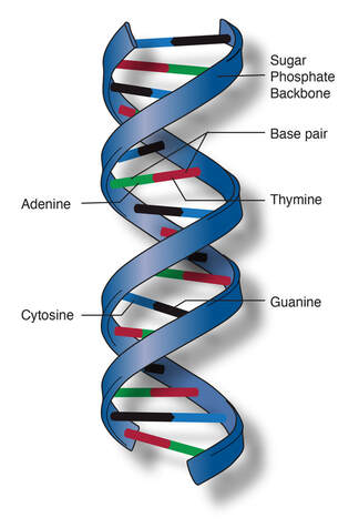 Schematic of the double helix. Credit: National Human Genome Research Institute. Schematic of the double helix. Credit: National Human Genome Research Institute. It is latter feature on which I want to briefly comment. In all eukaryotic organisms (organisms with complex cells, which effectively means everything except bacteria) DNA is arranged as linear threads organised in structures called chromosomes which are located in the cell’s nucleus. Further, as was shown when I was a student, the sub-cellular compartments known as mitochondria (which carry out ‘energy metabolism’) and in plant cells, chloroplasts (which carry out photosynthesis) contain their own DNA (as befits their evolutionary origin – see the book (1)). However, there has been debate for many years as to whether there are any other types of DNA in animal or plant cells. Indeed, I can remember discussing, many years ago, a research project which it was hoped would answer this question. Obviously if a cell is invaded by a virus, then there will be, at least temporarily, some viral genetic material in the cell but as for the question of other forms of DNA, there has been no clear answer.  Labelled electron micrograph of a plant cell showing nucleus, mitochondria and chloroplasts. Credit: H. J. Arnott and Kenneth M. Smith. Labelled electron micrograph of a plant cell showing nucleus, mitochondria and chloroplasts. Credit: H. J. Arnott and Kenneth M. Smith. Which brings me to a recent article in The Guardian newspaper (2). Scientists have known for some time that some cancers are caused by specific genes called oncogenes (3). It has now been shown that some oncogenes can exist, at least temporarily, independent of the DNA strands that make up our chromosomes. In this form, they act like 'Bond villains' (4) according to some of the scientists who work on this subject, leading to formation of cancers that are resistant to anti-cancer drugs. In order to prevent such cancers we now need to find out how these oncogenes or copies thereof can 'escape' from chromosomes to exist as extra-chromosomal DNA. I would also suggest that they may be deactivated by targeted gene editing.
John Bryant Topsham, Devon February 2023 (1) Graham Swinerd and John Bryant, From the Big Bang to Biology: where is God?, Kindle Direct Publishing, 2020, Chapter 5 (2) ‘Bond villain’ DNA could transform cancer treatment, scientists say. Cancer Research, The Guardian newspaper. (3) Oncogenes are mutated versions of genes that normally have a regulatory role in cell proliferation. When mutated they promote unregulated cell proliferation. They occur in all vertebrate animals and homologous sequences have been found in fruit flies. (4) The villains in James Bond films are often both sinister and subtle. John writes … ‘Save the planet!’ is one of the slogans in campaigns that encourage governments to aim, as soon as possible, for ‘net zero’ carbon dioxide emissions. However, planet Earth itself does not need to be saved. As we discuss in Chapter 8 of the book, it been through many climatic fluctuations in its 4.6 billion-year history and it is a testament to its survival of those ups and downs that we are here to talk about it. Leaving aside the extreme temperature fluctuations of the very young Earth and focussing ‘only’ on the 3.8 billion years during which there has been life on the planet, it is clear that Earth has had periods of being significantly warmer than now. Thus, it has been calculated that in the Cretaceous the average global temperature was at least 12°C higher than at present and there is evidence that trees grew on Antarctica and on land within the Arctic Circle. By contrast, Earth’s overall climate is at present cooler than average and has been so for about half a million years. The name for this is an Ice Age. The climate is characterised by alternation of very cold glacial periods (often called ‘ice-ages’ in colloquial usage), of which there have so far been five (the most recent ‘peaked’ about 22,000 years ago) and less cold interglacial periods, like the one that we are in now. 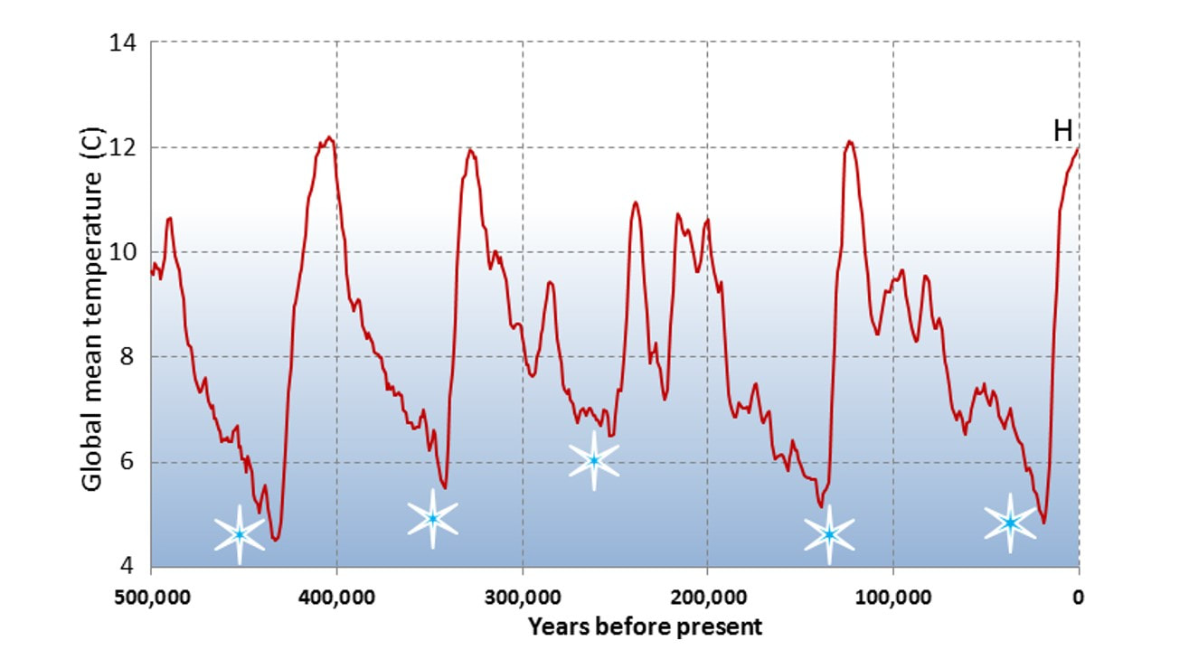 Glacial and inter-glacial interludes in the current Ice Age. Credit: from Steven Earle (1). Each of the varying climatic eras in Earth’s history has been characterised by its own particular ‘balance of nature’ in which the atmosphere, geosphere, hydrosphere and biosphere are in a dynamic equilibrium, as described in James Lovelock’s Gaia hypothesis. If physical conditions on Earth change dramatically, then, in the words of Lovelock ‘Gaia is re-set’ or in other words, a new dynamic equilibrium is established.  James Lovelock on his 100th birthday. Credit: The Science Museum. However, that equilibrium may be ‘challenged’ by phenomena such as volcanic eruptions which push a lot of carbon dioxide into the atmosphere. I was therefore very interested to read a recent article in New Scientist (2) which reported on research at Pennsylvania State University showing that the resulting increase in temperature would be countered by an increase in the rate of weathering and erosion of particular types of rock. This would lead, via a series of simple chemical reactions, to the carbon dioxide being trapped as ‘carbonate minerals’. The scenery at Guilin in southern China is made of types of rock whose weathering is thought to have contributed to this process. The author spoke of the system as a sort of coarse thermostat but added that it works too slowly to ameliorate the current rate of increase in the concentration of atmospheric carbon dioxide.  Guilin, China. Credit: John Bryant ‘Modern’ humans, Homo sapiens, have only been around for a very brief segment of the Earth’s long history. Our species arose in Africa about 250,000 years ago, when the third of the recent series of glaciations that I mentioned earlier was at or near its peak. From those origins in Africa, humans spread out to inhabit nearly the whole of the planet; human culture, society and then technology, grew and flourished. Humans are clearly the dominant species on Earth. Nevertheless, we can identify times in our history when climate would have made habitation of some areas impossible, namely the glacial interludes referred to above. Although modern technology makes it possible to live, after a fashion, on land covered in several metres of ice, that was not true 30,000 years ago. Thus, we can envisage climate-driven migration of both humans and Neanderthals, moving towards the equator as the last glacial interlude held the Earth in its icy grip. Returning to the present day, even the relatively modest (in geo-historical terms) increase in temperature that is currently being caused by burning fossil fuels is very likely to drive human migration. Some of this will be a result of an indirect effect of rising temperatures, namely the rising sea level (see next paragraph) but some will occur because there are regions of the world where, if temperature rise is not halted, the climate itself and the direct effects thereof will make human habitation more or less impossible. My colleague at Exeter University, Professor Tim Lenton, has been part of a team doing the detailed modelling, one of the results of which is this map which predicts the extent of uninhabitable zones in the year 2070 if we adopt a ‘business as usual’ approach to climate (3). I will leave our readers to think about the implications of this. 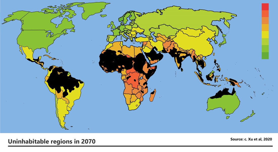 Zones on Earth that will be uninhabitable (marked in black). In the previous paragraph I briefly mentioned rising sea levels. The increase so far has been, on average, about 17 cm which at first sight seems quite small. However, it is large enough to have increased the frequency of coastal flooding in low-lying coastal regions. Thus, much of, for example, Bangladesh (4) (including half of the Sundarbans (5), the world’s largest mangrove forest) is highly vulnerable, as are many Pacific islands. Some island communities are already planning to leave and to rebuild their communities, including all their traditions and folk-lore, in less flood-prone locations. The islanders will be a part of the 600 million sea-level-refugees projected to be on the move by the end of this century, in addition to those moving away from the uninhabitable zones mentioned above.  The Sundarbans National Park. Credit: juggadery/Flickr via Wikimedia Commons. The rise in sea level is and will be caused by the melting of Arctic ice, including the Greenland ice-sheet and especially by the melting of Antarctic ice. Thinking about this reminded me of an article in The Guardian newspaper in 2020 (6). In order to illustrate this, I would like you to take an ice-cube out of your freezer (probably at -18°C) and place it at ‘room’ temperature (probably somewhere between 15 and 18°C). It does not melt instantly – and indeed, may last, depending on its size and the actual room temperature, a couple of hours. And so it is with environmental ice. In terms of the rise in sea level attributable to global warming, ‘we ain’t seen nothin’ yet’. The author of the article, Fiona Harvey, states, based on a paper in the scientific journal Nature, that even if we manage to keep the overall rise in temperature to 2°C, Antarctic ice will go on melting well into the next century and will raise sea levels not by a few cm but by about 2.5 metres, a scenario that hardly bears thinking about. Dealing with climate change and the knock-on effects thereof is thus a matter of extreme urgency. 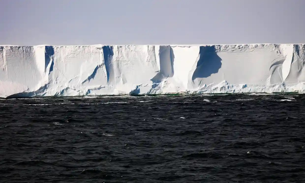 The Antarctic Ice Sheet. Credit: imageBROKER/Alamy Stock Photo via The Guardian. John Bryant Topsham, Devon January 2023 (1) Steven Earle, Physical Geology (2nd Edition), 2019. Physical Geology - Open Textbook (opentextbc.ca)
(2) Rock weathering ‘thermostat’ is too slow to prevent climate change | New Scientist (3) Future of the human climate niche | PNAS (4) Intense Flooding in Bangladesh | nasa.gov and Introduction to Bioethics (Bryant and la Velle, 2018) p 298. (5) The Sundarbans straddles the India/Bangladesh border. (6) Melting Antarctic ice will raise sea level by 2.5 metres – even if Paris climate goals are met, study finds | Climate crisis | The Guardian 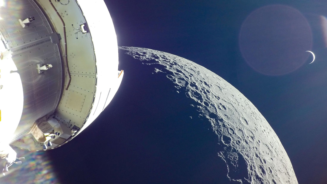 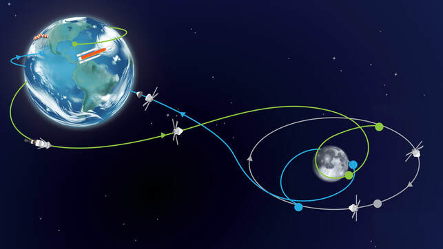 Graham writes … After a number of frustrating delays, the uncrewed, moon orbiting, test mission designated Artemis 1 finally got off the launchpad on 16 November 2022. You may recall that one of these delays was not insignificant, due to the arrival of Hurricane Ian which caused a return of the launch vehicle to the shelter of the Vehicle Assembly Building. The mission lasted about three and half weeks, finally splashing down in the Pacific Ocean on 11 December 2022. The objectives of the mission were achieved, the principal one being to test out the Orion spacecraft systems, prior to the future launch of crewed missions. The mission profile is rather more elaborate than that of the Apollo missions, as illustrated by the accompanying graphic. This blog post is essentially a picture gallery of aspects of the mission. In retrospect, I realised that the beautiful blue orb of the Earth features significantly in my choice of images. Also many of the images are ‘selfies’, showing elements of the spacecraft. This is achieved by using imagers attached to the spacecraft’s solar panels. All images are courtesy of NASA. I hope you enjoy the beauty and grandeur of God's creation in what follow ...! 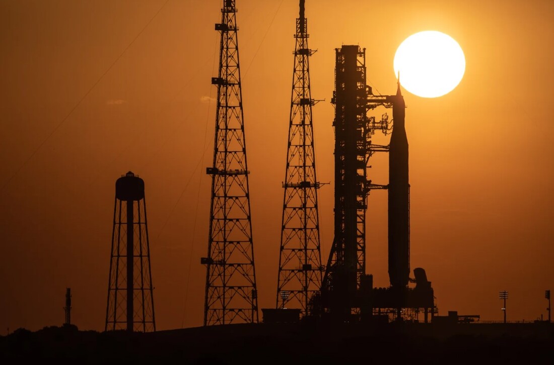 1. The Artemis 1 Space Launch System on the pad.  2. A close up of the Orion spacecraft in launch configuration, with launch escape tower attached.  3. Spectators watch Artemis 1 as it makes its way to orbit (16 November 2022).  4. Orion’s camera looks back on ‘the good Earth’ as the vehicle makes its way to the moon. The picture is captured by a ‘selfie stick’ installed on one of the solar panels. The image also shows the European service module’s propulsion system, featuring the main orbit transfer engine, the smaller trajectory adjustment thrusters, and, smaller still, the attitude control thrusters. One of the solar panels is prominent.  5. Approaching the moon. 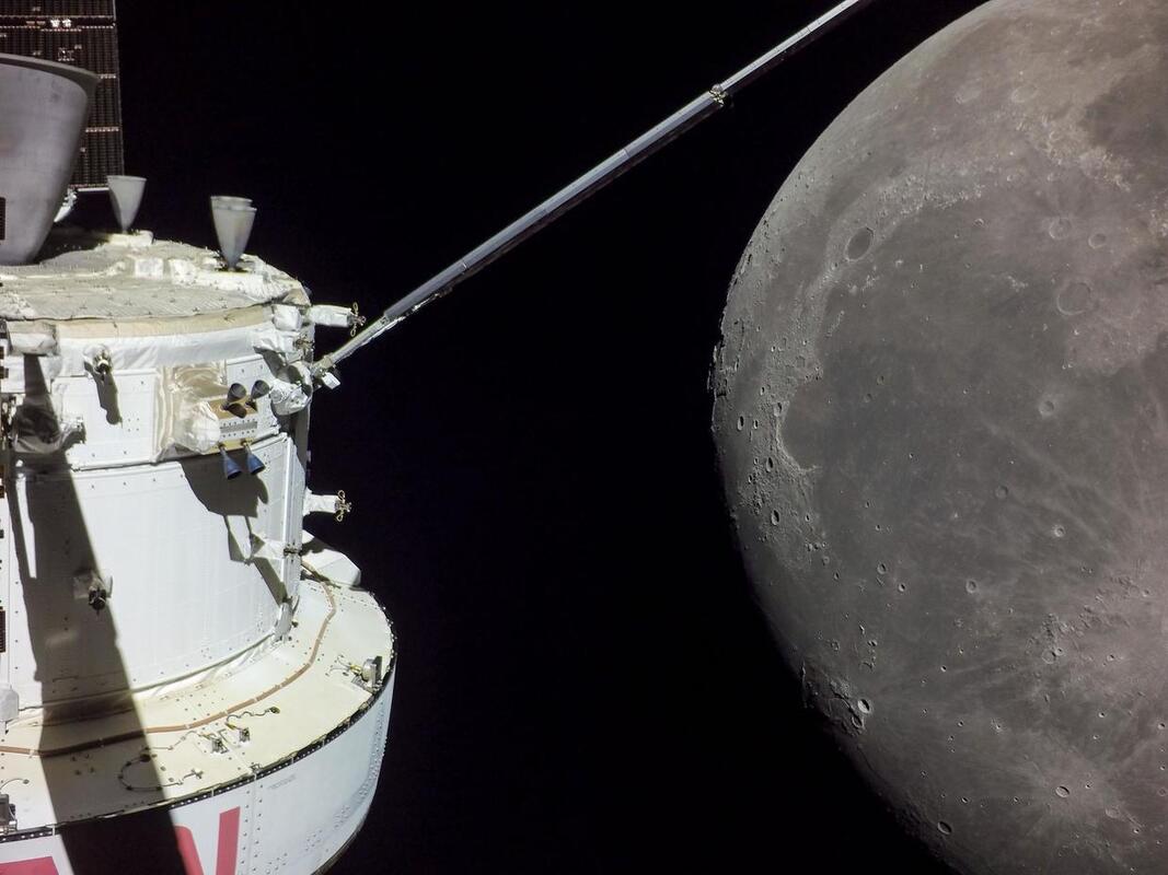 6. Lunar surface detail captured during the close powered swingby.  7. Lunar surface detail captured during the close powered swingby.  8. The Earth and the moon can be seen beyond the conical crew capsule. The large structural collar at its base provides protection for the capsule’s heatshield. 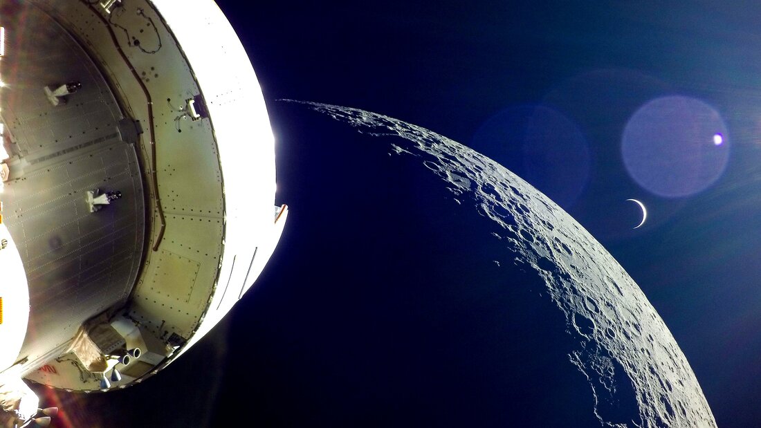 9. Crescent Earth and crescent moon from Orion. A striking and beautiful picture, perhaps reminiscent of an ‘Apollo 13’ film poster! 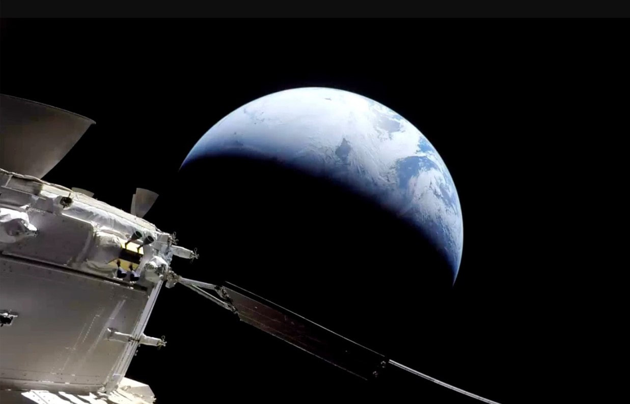 10. The Earth looms large again as Orion races towards atmospheric re-entry.  11. Parachute landing after a successful re-entry (11 December 2022). 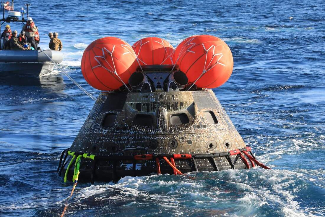 12. Capsule recovery led by USS Portland. So, after the successful flight of Artemis 1, what does the future hold? In contrast to the ‘manic’ flight schedule of the Apollo programme leading up to the first landing in July 1969, the Artemis schedule is frustratingly more relaxed! The next event is the launch of Artemis 2, which is planned for May 2024. This will be the first crewed mission of the Orion system with a planned duration of 10 days. Note that we no longer refer to ‘manned’ missions, as the upcoming flights will involve the participation of lady astronauts! This second flight will take people out to a flyby of the moon, thus giving the system a thorough test with people on board. 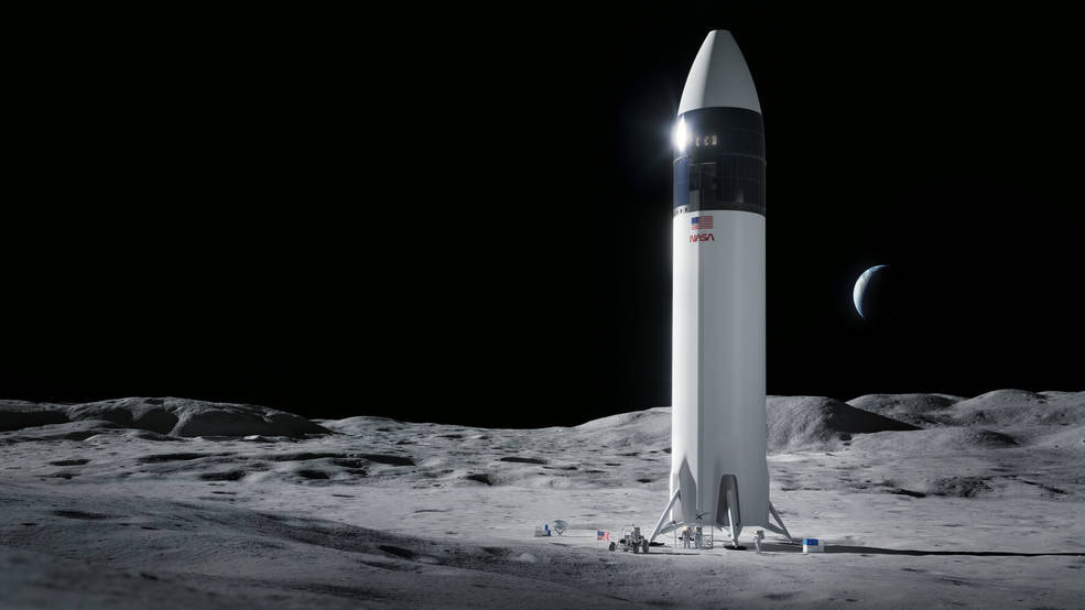 An artist's impression of the SpaceX Starship HLS on the lunar surface, planned for 2025. Then, planned for 2025, the Artemis 3 mission will land astronauts on the moon for the first time since Apollo 17 in 1972. To supply the flight infrastructure to transfer astronauts from lunar orbit to the moon’s surface, and back, NASA have contracted the private company SpaceX. In recent times, this enterprise has proved itself in supplying a reliable transfer system, taking astronauts to and from the Earth-orbiting International Space Station. SpaceX proposes using a lunar landing variant of its Starship spacecraft, called the Starship HLS (Human Landing System). See the image above, showing an artist’s impression of the SpaceX HLS on the lunar surface – a monstrous vehicle in comparison to the Apollo era Lunar Excursion Module. There seems to be a lot of questions as to why NASA has chosen this route, but that’s a story for another time!
Graham Swinerd Southampton January 2023  Credit: www.protothema.gr John writes … The past few months have seen announcements of several new medical treatments based on manipulating DNA. I want to highlight just a couple of these which illustrate how techniques developed in research labs are helping doctors to use knowledge about genes and genetics to treat conditions which had previously been incurable.  Credit: Goodreads Credit: Goodreads The first concerns haemophilia, a condition in which blood fails to clot. It is caused by the absence of a protein involved in the clotting process which is in turn caused by a mutation in the gene encoding that protein. In 85% of haemophilia cases, it is Factor VIII that is missing. This particular mutation is famous because of its presence in Queen Victoria’s family, as described beautifully in Queen Victoria’s Gene by D.M. and W.T.W. Potts. The remaining 15% of cases involve a different clotting factor, Factor IX, and are again caused by a mutation in the relevant gene. Both conditions are suitable targets for somatic cell gene therapy in which the cells that make the protein – both these factors are made in the liver – are supplied with a functional copy of the gene. But, despite the basic simplicity of that process, achieving it is much more difficult, as my students have often heard me say. Indeed, despite early optimism, treating Factor VIII deficiency via gene therapy has not yet been achieved. However, there has been success in treating the rarer condition, Factor IX deficiency, as reported by the BBC back in the summer: Transformational therapy cures haemophilia B – BBC News. The process is relatively simple. The gene encoding Factor IX is inserted into an engineered harmless adenovirus which can make itself at home in the liver and thus deliver the desired gene to the liver cells. One person, Elliott Mason (pictured below), who has undergone this treatment, which, for the patient, involves a one-hour infusion of the engineered virus into the liver, said that it was astonishing to see that his Factor IX levels had gone from 1% of normal to being in the normal range. He added "I've not had any treatment since I had my therapy, it's all a miracle really, well it's science, but it feels quite miraculous to me." The team of scientists and doctors involved in developing this treatment believes that the patients who received it will not need another gene infusion for at least eight years.  Elliot Mason My second example is successful treatment of T-cell acute lymphoblastic leukaemia which had resisted all other treatments. Earlier this month, doctors at the world-famous Great Ormond Street Hospital in London (www.gosh.nhs.uk) announced a ‘first’ in that they had used DNA base-editing to cure a 13-year-old girl, Alyssa, of her leukaemia: see Base editing: Revolutionary therapy clears girl’s incurable cancer – BBC News. I’ll explain what they did later in this post but for the minute I want to go back seven years. DNA base-editing is a very precise and sophisticated form of genome editing. Genome editing was used in 2015, also at Great Ormond Street, to treat a baby, Layla Richards, with an equally resistant acute lymphoblastic leukaemia. The technique was completely new; it had never been used on a human patient but the local medical ethics committee readily gave permission for its use because without it, the little girl was certain to die. As I have previously described (1), donated T-cells (T-cells are the immune system’s hunters) were subjected to very specific and targeted genetic modification and genome editing to enable them to hunt down and eradicate the cancer cells. The modified T-cells were infused into Layla and within two months she was completely cancer-free. Building on this success, the team used the same technique a few months later to treat another very young leukaemia patient (2). Returning to the present day, the team treating Alyssa again used donated T-cells. These were then modified by DNA base-editing as shown in the diagram below. 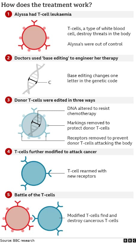 As with the earlier treatments, a genetic modification was also required to enable the edited T-cells to bind to and destroy the cancerous T-cells. Alyssa is part of a trial that also includes nine other patients but she is the first for whom results of the treatment are available. She says ‘"You just learn to appreciate every little thing. I'm just so grateful that I'm here now. It's crazy. It's just amazing [that] I've been able to have this opportunity, I'm very thankful for it and it's going to help other children, as well, in the future.”
One of the inventors of DNA base-editing, Dr David Lui, was delighted that the technique had been used in this life-saving way: “It is a bit surreal that people were being treated just six years after the technology was invented. Therapeutic applications of base-editing are just beginning and it is humbling to be part of this era of therapeutic human gene-editing." John Bryant Topsham, Devon. December 2022 (1) Introduction to Bioethics, 2nd edition, John Bryant and Linda la Velle, Wiley, 2018. p139. (2) Two baby girls with leukaemia ‘cured’ using gene-editing therapy – Genetic Literacy Project.  There is a time for everything and a season for every activity under the heavens … (Ecclesiastes 3, v1) He has made everything beautiful in its time. He has also set eternity in the human heart … (Ecclesiastes 3, v11) John writes … I quoted these verses at the front of my PhD thesis many years ago. They sandwich a passage in which ‘[there is] a time to …’ as used in the folk song ‘Turn, turn, turn.’ Many people have some familiarity with at least part of the passage without knowing that it comes from the Bible. The version of ‘Turn, turn, turn’ recorded in 1966 by Pete Seeger was recently played on BBC radio. It was obvious that the programme’s presenter was one of those who do not know that the words are Biblical – he ascribed them to the anti-war movement of the 1960s.  In recent days I have gone back to these verses and again thought about them in relation to the creation. The existence of seasons results from the way our planet is set up but it doesn’t have to be that way. Planets without seasons are perfectly good planets. So, as I enjoy the lovely autumn colours and indeed understand the underlying biology, I thank God that He has made everything beautiful in its time.  But that also challenges me. Autumns are getting warmer; the biological changes, except those driven entirely by day-length, are occurring later. Ecosystems are changing because the climate is changing; this is a matter for prayer and urgent action.  John Bryant
Topsham, Devon November 2022 All pictures are credited to the author.  Graham writes … In October’s post, John discussed the winner of the Nobel Prize of Physiology and Medicine, and this month I’d like to say something about the work of the winners of the Physics Prize, and the extraordinary things it says about the nature of reality. There were three winners, Alain Aspect, John Clauser and Anton Zeilinger, and broadly speaking they earned the prize for their work on the topic of quantum entanglement. So what is quantum entanglement, and why is it important? I’d like to say something about this concept, hopefully in language that is accessible to non-physicists As you may know, prior to the 1900s, the laws devised by Isaac Newton reigned supreme. It is also fair to say that for many engineering and science applications today, Newton’s theory still works. This classical theory is elegant, compact and powerful, and is still part of the education of a young science student today. One of the main aspects of Newton’s physics is what it says about the nature of reality. Put simply, if you tell me how the world is now, then the theory will tell you precisely how the world will be tomorrow (or indeed yesterday). In other words, if the positions and velocity of all the particles in the Universe were known at a particular time, then in principle Newton will be able to determine the state of all the particles at another time. This total determinism is a defining facet of Newtonian physics. However, in the early years of the 20th Century, the comforting edifice of classical physics collapsed under the onslaught of a new theory. Physicists investigating the world of the very small – the realm of molecules, atoms and elementary particles – found that Newton’s laws no longer worked. A huge developmental effort on the part of scientists, such as Einstein, Planck, Bohr, Heisenberg, Schrödinger and others, ultimately led to an understanding of the micro-world through the elaboration of a new theory called quantum mechanics (QM). However, it was soon realised that the total determinism of classical physics was lost. The nature of reality had changed dramatically. In the new theoretical regime, if you tell me how the world is now, QM will tell you the probability that the world is in this state or in that.  Albert Einstein. Credit: NobelPrize.org Albert Einstein. Credit: NobelPrize.org Einstein was one of the principal founders of the theory of QM, but it is well known that over time he came to reject it as a complete description of the Universe. Much has been made of Einstein’s resistance to QM, summed up by his memorable quote that “God does not play dice with the world”. However, Einstein could not deny that QM probabilities provided a spectacularly accurate prediction of what was going on in the microworld. Instead, he believed that QM was a provisional theory that would ultimately be replaced by a deeper understanding, and the new theory would eliminate the probabilistic attributes. He could not come to terms with the idea that probabilities defined the Universe, and felt there must be an underlying reality that QM did not describe. He believed that this deeper understanding would emerge from a new theory involving what has become known as ‘hidden variables’. On a personal note, I have to say I have great sympathy with Einstein’s view. As an undergraduate, with a very immature appreciation of QM, I too could never get to grips with it from the point of view of its interpretation of how the Universe works. This is one of the reasons why I studied general relativity – Einstein’s gravity theory – at doctorate level, which is inherently a classical theory.  Getting back to the discussion, Einstein strived to find his ultimate theory until the end of his life. Along the way, he was always attempting to find contradictions and weaknesses in QM. If he believed that he had found something, he would throw out a challenge to his circle of eminent ‘QM believers’. This stimulating discourse continued for many years. Then in 1935, with the publication of a paper with coauthors Podolsky and Rosen, Einstein believed he had found the ultimate weakness in QM in a property referred to as quantum entanglement (QE). This publication became known as the ‘EPR paper’. In broad terms, QE can be summarised along the lines of – if two objects interact and then separate, a subsequent measurement of one of them revealing some attribute would have an instantaneous influence on the other object regardless of their distance apart.  You might ask, why does this have such a profound impact on our understanding of reality? To grasp this, we need to discuss in a little more detail what this means when we consider quantum objects, like subatomic particles, and their quantum qualities, such a quantum spin. We have discussed the enigma of quantum spin before (see the March 2022 blog post). If we measure the quantum spin of a particle about a particular axis, then the result always reveals that it is spinning either anti-clockwise or clockwise (as seen from above), with the same magnitude. The former state is referred to ‘spin up’ and the latter ‘spin down’. There are just two outcomes, and this is a consequence of the quantised nature of the particle’s angular momentum (or rotation). As I have said before – nobody said quantum spin was an intuitive concept! It is possible to produce two particles in an interaction in the laboratory such that they zoom off in opposite directions, one in a spin up state and the other in a spin down state (for example). In the process of their interaction the two particles have become entangled, and we can measure their spin in detectors placed at each end of the laboratory. Another part of this story is understanding the nature of measurement in QM. In the example we have chosen above, the conventional interpretation of QM says that the particle’s spin state is only revealed when a measurement takes place. Prior to this moment the particle is regarded as being in a state in which it is neither spin up nor spin down, but in a fuzzy state of being both. The probability of one or other state is defined by something called the wave function, and a collapse of the wave function occurs the moment a measurement is made, to reveal the actual spin state of the particle. This process is something of a mystery, and is still not fully understood. However, that is another story. For interested readers, please Google ‘the collapse of the wave function’ for more detail. So, in our discussion, we have two ways of interpreting our experiment. That of QM which says that the spin state of the particle is only revealed when a measurement is made, and that of Einstein who believed in an underlying reality in which the spin state has a definite value throughout. If you think about the two entangled particles created in the lab, discussed above, then QE only presents us with an issue if QM is correct and Einstein is wrong. In this case, the measurement of the spin of one particle reveals its value (up or down), and an instantaneous causal influence will reveal the state of the other (the opposite value), even if the two particles are light years apart. Einstein called this "strange spooky action at a distance”, and it troubled him deeply, particularly as both his theories of relativity forbid instantaneous propagation of any physical influence. QM could not, in his view, give a full final picture of reality. For years, nobody paid much attention to the EPR paper, mostly because QM worked. The theory was successful in explaining physics experiments and in technology developments. Since no one could think of a way of testing Einstein’s speculation that one day QM would be replaced by a new theory that eliminated probability, the EPR paper was regarded merely as an interesting philosophical diversion.  John Stuart Bell. Credit: CERN John Stuart Bell. Credit: CERN Einstein died in 1955, and the debate about QE seemed to die with him. However, in 1964 an Irish physicist called John Stuart Bell proved mathematically that there was a way to test Einstein’s view that particles always have definite features, and that there is no spooky connection. Bell’s simple and remarkable incite was that doable experiments could be devised that would determine which of the two views is correct. Put another way, Bell's theorem asserts that if certain predictions of QM are correct then our world is non-local. Physicists refer to this ‘non-locality’ as meaning that there exist interactions between events that are too far apart in space and too close together in time for the events to be connected even by signals moving at the speed of light. Bell’s theorem has been in recent decades the subject of extensive analysis, discussion, and development by both physicists and philosophers of science. The relevant predictions of QM were first convincingly confirmed by the experiment of Alain Aspect (one our Nobel Prize winners) et al. in 1982, and they have been even more convincingly reconfirmed many times since. In light of these findings, the experiments thus establish that our world is non-local. I emphasise once again that this conclusion is very surprising, given that it violates the theories of relativity, as mentioned above. 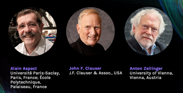 The Nobel Prize winners for 2022. Credit: Optica In summary then, this year’s Nobel Prize for Physics has been awarded to Alain Aspect, John Clauser and Anton Zeilinger, whose collective works have used Bell’s theorem to establish to most people’s satisfaction (1) that Einstein’s conventional view of reality is ruled out (2) that quantum entanglement is real and (3) that quantum mechanics and quantum entanglement can be used to develop new technologies (such as quantum computing and quantum teleportation).
Usually, the Nobel Physics Prize is awarded to scientists whose work makes sense of Nature. This year’s laureates reveal that the Universe is even stranger than we thought, and in addition they achieved the rarest of things – they proved Einstein wrong! Graham Swinerd Southampton, UK November 2022 |
AuthorsJohn Bryant and Graham Swinerd comment on biology, physics and faith. Archives
May 2024
Categories |
 RSS Feed
